


ABSTRACT
The fraction of active galactic nucleus (AGN) luminosity obscured by dust and re-emitted in the mid-IR is critical for understanding AGN evolution, unification, and parsec-scale AGN physics. For unobscured (Type 1) AGNs, where we have a direct view of the accretion disk, the dust covering factor can be measured by computing the ratio of re-processed mid-IR emission to intrinsic nuclear bolometric luminosity. We use this technique to estimate the obscured AGN fraction as a function of luminosity and redshift for 513 Type 1 AGNs from the XMM-COSMOS survey. The re-processed and intrinsic luminosities are computed by fitting the 18 band COSMOS photometry with a custom spectral energy distribution fitting code, which jointly models emission from hot dust in the AGN torus, from the accretion disk, and from the host galaxy. We find a relatively shallow decrease of the luminosity ratio as a function of Lbol, which we interpret as a corresponding decrease in the obscured fraction. In the context of the receding torus model, where dust sublimation reduces the covering factor of more luminous AGNs, our measurements require a torus height that increases with luminosity as  . Our obscured-fraction–luminosity relation agrees with determinations from Sloan Digital Sky Survey censuses of Type 1 and Type 2 quasars and favors a torus optically thin to mid-IR radiation. We find a much weaker dependence of the obscured fraction on 2–10 keV luminosity than previous determinations from X-ray surveys and argue that X-ray surveys miss a significant population of highly obscured Compton-thick AGNs. Our analysis shows no clear evidence for evolution of the obscured fraction with redshift.
Export citation and abstract BibTeX RIS
1. INTRODUCTION
The spectral energy distribution (SED) of active galactic nuclei (AGNs) covers the full electromagnetic spectrum from radio to hard X-rays. The most prominent features are the "near-infrared bump" at ∼10 μm and an upturn in the optical–UV, the so-called "big-blue bump" (BBB; Sanders et al. 1989; Elvis et al. 1994, 2012; Richards et al. 2006; Shang et al. 2011; Krawczyk et al. 2013). The BBB is thought to be representative of the emission from the accretion disk around the supermassive black hole (SMBH), while the near-infrared bump is due to the presence of dust that re-radiates a fraction of the optical–UV disk photons at infrared wavelengths.
The presence of this screen of gas and dust surrounding the accretion disk is the foundation of the unified model for AGNs (Antonucci 1993; Urry & Padovani 1995), according to which the observed AGN SED shape arises from different viewing angles relative to the obscuring material, under the simple assumption that the dust is smoothly distributed in a toroidal shape. This gives rise to the classification distinction between unobscured (Type 1) AGNs and obscured (Type 2) AGNs. In the former case, the observer has a direct view into the nuclear accretion disk region, while in the latter the optical–UV emission is completely or partially extincted depending on the inclination angle. A key ingredient of this model is the spatial distribution of this dust, which governs the amount of obscuration. This can be parameterized by a dust covering factor and its dependence on nuclear luminosity. In the simplest model where the obscuring medium is a dusty torus, this covering fraction is directly related to the opening angle of the torus, or equivalently its height and distance from the nucleus. AGN unification postulates that the disk and broad-line region emit anisotropically toward the observer for a Type 1 AGN while, in the optically thin case, the re-processed optical–UV emission is re-radiated isotropically in the infrared. For a toroidal distribution of dust, the mid-infrared luminosity is altered by inclination effects as well (Dullemond & van Bemmel 2005; Granato & Danese 1994).
Thus, the ratio of mid-infrared to bolometric luminosity, which we define as R, provides an estimate of the covering factor of the dust; therefore, it is used to infer the fraction, fobsc, of AGNs that are obscured. The parameter fobsc is a function of the luminosity ratio R, and in the simplest model where the torus is optically thin to its own infrared radiation (see Granato & Danese 1994 and our detailed discussion in Section 6.1), it can be written as

In this paper, we estimate R for a large sample of X-ray-selected Type 1 AGNs, which is used to determine fobsc. Note that the terms covering factor and obscured fraction refer to the same physical quantity, and the amount of AGN obscuration is equivalent to R in the optically thin case only (see also Section 2.5 in Nenkova et al. 2008a).
In the context of AGN unification, the obscured fraction fobsc is simply a free parameter, and unification makes no prediction for its dependence on luminosity, although there are compelling physical arguments for why such a relationship might exist. In more luminous AGNs the distance of the torus from the central source is larger; hence, the opening angle (defined as the minimum angle between the perpendicular to the disk and a line of sight that intersects the torus; see Figure 1 in Simpson 1998) is also larger, assuming a constant height of the torus. Dust grains in the inner part of the torus are heated by the primary optical–UV continuum radiation and destroyed by evaporation; hence, the torus extends from the dust sublimation radius outward (Barvainis 1987; see also Hönig & Beckert 2007). We therefore expect a decrease of fobsc with increasing luminosity. This is the so-called receding torus model (Lawrence 1991).
Another explanation of AGN obscuration does not involve the presence of the dusty torus, but rather a parsec-scale wind/outflow. In this scenario the torus is identified with the outer region of a hydromagnetic disk-driven outflow (Konigl & Kartje 1994; Elitzur & Shlosman 2006; but see also the recent works done by Dorodnitsyn et al. 2011; Dorodnitsyn & Kallman 2012). Such winds can also provide an important link between SMBH and host galaxy (i.e., AGN feedback). From a theoretical point of view, initial attempts to model the AGN torus have assumed a smooth dust distribution (Pier & Krolik 1992; Granato & Danese 1994; van Bemmel & Dullemond 2003), but such prescription fails to fully reproduce the mid-infrared SED. Nenkova et al. (2002, 2008b) suggest that a clumpy distribution better represents the observations, with average covering factor value of ∼0.6. Thus, an empirical calibration of the amount of re-processed optical–UV emission, and its dependence on luminosity, would greatly inform theoretical models of parsec-scale physics and the environment of AGNs.
Broadly speaking, there is mounting evidence that SMBHs may be characterized by significant differences in their accretion processes, triggers, and environment as a function of luminosity and/or cosmic time (Hopkins et al. 2007). According to the classic Soltan argument (Soltan 1982), the luminosity density of AGN emission over the history of the universe should be commensurate with the local mass density of SMBHs. However, this commensurability requires that the census of cosmic AGN accretion accounts for the amount of obscured accretion, which can depend on both luminosity and cosmic time. The amount of obscuration is therefore a fundamental ingredient in order to understand the formation history of SMBHs (Hopkins et al. 2007).
The AGN obscured fraction can be determined via multiple independent methods. One is to use AGN demographics, that is, by conducting a census of AGNs at a wavelength that is agnostic to viewing angle (such that both Type 1 and Type 2 AGNs are selected) and then simply computing the obscuring fraction as fobsc ≃ NType-2/(NType-1 + NType-2). Such determinations typically require spectroscopic follow-up to distinguish Type 1 (broad-line) from Type 2 (narrow-line) AGNs, but if multi-wavelength data are available, an SED-based classification can be adopted. The amount of obscuration is also a crucial ingredient for models of the cosmic X-ray background (XRB; Gilli et al. 2007). Indeed, the XRB amplitude and spectral shape depend on the relative contributions of unobscured, moderately obscured (Compton-thin), and highly obscured (Compton-thick) AGNs. Thus, XRB synthesis models that attempt to reproduce observations of the XRB give another independent estimate of the obscured fraction given assumptions about the Compton-thin populations. Finally, the obscured fraction can be determined from an analysis of AGN SEDs, because the ratio of the reprocessed infrared luminosity to bolometric AGN emission depends on the covering factor of the obscuring medium (e.g., Maiolino et al. 2007, hereafter M07; Treister et al. 2008; Sazonov et al. 2012). It is the latter approach that we pursue in this paper.
The first evidence for a luminosity-dependent obscured fraction was reported in Lawrence & Elvis (1982), where fobsc is parameterized by the hard-to-soft X-ray luminosity ratio (L[2–10] keV/L[0.5–2] keV), while Ueda et al. (2003) first measured a significant decrease in the fraction of obscured AGNs with increasing X-ray luminosity, by employing a demographic approach (similar results have been obtained, with the same methodology, from independent X-ray-selected AGN samples by Steffen et al. 2003; Hasinger 2004; La Franca et al. 2005; Treister & Urry 2006; Hasinger 2008; Merloni et al. 2013). The obscured fraction in these studies decreases from 0.8 to 0.1, with L[2–10] keV increasing from 1042 erg s−1 to 1046 erg s−1. Demographic analyses, employing optically selected samples from the Sloan Digital Sky Survey (SDSS; Simpson 2005) and radio-selected AGN samples (Grimes et al. 2004), have found a similar trend between fobsc and [O iii] luminosity, with an obscured fraction decreasing from 0.85 to 0.5 with increasing [O iii] luminosity (1044–46 erg s−1; see also Willott et al. 2000 for similar results by employing the [O ii] emission-line luminosity). The demographic analysis presented by Assef et al. (2013) for a sample of WISE-selected AGNs in the Bo tes field confirms that a relation between the Type 1 AGN fraction and the AGN bolometric luminosity also exists. The Type 1 AGN fraction estimated by Assef et al. (2013) ranges from ∼0.3 to ∼0.64 with Lbol = 1044.3–45.6 erg s−1, which can be translated into an obscured fraction decreasing from 0.7 to 0.36 with increasing Lbol.
Inherent in all of these demographic studies are ambiguities in how Type 1/2 AGNs are identified and defined, and therefore their selection of AGNs could be biased. For example, X-ray surveys miss Compton-thick AGNs as pointed out by Gilli et al. (2007), where, although the fraction of obscured AGNs is assumed to decrease with X-ray luminosity, a non-negligible population of obscured AGNs is still required to properly model the XRB spectrum. Optical selection of Type 2 AGNs may miss obscured objects that do not show strong narrow emission line regions (Reyes et al. 2008), while radio-loud objects might have different obscured fraction than radio-quiet ones in radio-selected AGN samples (Willott et al. 2000).
Previous work using SED-based analyses to constrain the obscured fraction has been performed by several studies using AGN samples selected from SDSS (e.g., Gallagher et al. 2007; Hatziminaoglou et al. 2008; Roseboom et al. 2013; Ma & Wang 2013) and Spitzer (e.g., M07; Treister et al. 2008; Hatziminaoglou et al. 2009). SED-based studies have found covering factors of the order of 0.3–0.4, considering optically selected AGN samples from SDSS (Roseboom et al. 2013) and the well-studied CLASXS Chandra survey (Rowan-Robinson et al. 2009). Spitzer-selected Type 1 AGN samples show average covering factors from hot dust clouds9 that range from 0.15 (Mor & Netzer 2012) to ∼0.4 (Rowan-Robinson et al. 2008; see also Hatziminaoglou et al. 2009 for a sample of Type 2 AGNs). All SED-based studies need photometric coverage over a broad range of wavelength, from infrared to optical–UV. Optical- and infrared-selected AGN samples did not have the X-ray coverage for a large number of objects. Therefore, in order to compare the results coming from X-ray analyses with infrared/optical ones, a bolometric correction (kbol) needs to be assumed. Corrections are also often assumed to estimate the total infrared and/or optical luminosity when the necessary multi-wavelength coverage is not present (e.g., M07; Treister et al. 2008). Very few studies, so far, have presented the obscured fractions corrected for the host galaxy emission, subtracting this component from the bolometric budget (see, for example, the recent work by Sazonov et al. 2012). However, even in these works, the specific assumptions about dust geometry and emission in the parameterization of covering factor are usually not discussed, and no reddening correction of the disk emission in the optical is applied.
The evolution of the AGN obscured fraction with redshift is even more uncertain. Ueda et al. (2003) did not find clear evidence for a redshift dependence (see also Gilli et al. 2007), while recently Hasinger (2008) has argued for a significant increase of the obscured fraction with redshift (Ballantyne et al. 2006; Treister & Urry 2006; but see also Gilli et al. 2010). Iwasawa et al. (2012) also show that the fraction of absorbed AGNs at high luminosity may be higher at high redshift than in the local universe considering a rest-frame 9–20 keV selection of heavily obscured AGNs at z > 1.7 from the deep XMM-CDFS survey (see also Vito et al. 2013 for similar results at z > 3).
The goal of the present study is to measure the covering factor of the AGN obscuring medium (i.e., the obscured fraction) and its dependence on luminosity and redshift. Our approach is to consider a sample of Type 1 AGNs, such that both optical–UV emission from the accretion disk and reprocessed infrared emission from the torus can be measured. The ratio of infrared to optical–UV luminosity can then be used to determine the covering factor of dust. We utilize SED fitting (Lusso et al. 2011, 2012, hereafter L11 and L12, respectively) to conduct a spectral decomposition of the various emission components in AGNs, and thus obtain a robust estimate of the nuclear and torus emission. We thus require a well-sampled SED over a broad range of wavelength. In particular, far-infrared data are fundamental to probe the star formation activity, while mid-infrared observations are necessary to cover the wavelengths where most of the re-processed AGN optical–UV luminosity is expected to be emitted. For these reasons, we carried out our analysis over a sample of Type 1 AGNs drawn from the XMM-COSMOS survey, which is a unique area given its deep and comprehensive multi-wavelength coverage: infrared coverage from Spitzer and Herschel; optical bands with Hubble, Subaru, SDSS, and other ground-based telescopes; near-UV (NUV) and far-UV (FUV) bands with the Galaxy Evolution Explorer (GALEX); and X-rays with XMM-Newton. Our approach exploits the best available multi-wavelength coverage, is less biased against Type 2 AGN classification inherent to demographic studies, and makes no assumptions about bolometric corrections since we directly fit the full AGN SED. Furthermore, our SED fitting approach explicitly corrects for the effect of intrinsic AGN reddening and subtracts off the contaminating emission from the host galaxy.
A comparison of our measurements of the obscured fraction with that determined independently from AGN demographics or synthesis of the XRB is interesting for several reasons. Naturally, these obscured fractions should all agree, but each approach depends on an independent set of assumptions. For example, as we will see in Section 6.1, the results of our SED fitting approach depend somewhat on the properties of the dust in the torus (e.g., optically thick or thin, anisotropic emission, etc.), which can thus be constrained by comparing to an independent determination from another technique. Demographic measurements of the obscured fraction require an unbiased survey of the total AGN population; hence, a disagreement with our SED-based obscured fraction estimates could reveal biases in these surveys. For example, X-ray surveys could be missing Compton-thick Type 2 AGNs, mid-IR selection could be severely contaminated by star-forming galaxies, and optical Type 2 AGN surveys might be missing sources lacking strong narrow line emission (see Merloni et al. (2013) for details about the dependency of the obscured fraction on the AGN classification).
The structure of this paper is as follows. In Section 2 we discuss the sample selection and the employed photometric data sets. In Section 3 we describe the SED fitting code and, in particular, the new developments with respect to L11 and L12. The luminosities computed at different wavelengths will be presented in Section 4. Our R estimates and their variation with Lbol are presented in Section 5, while the results of our analysis are discussed in Section 6. Conclusions are outlined in Section 7. Details regarding the SED fitting code and discussion about outliers are presented in the Appendix. We adopt a concordance Λ −cosmology with H0 = 70 km s−1 Mpc−1, ΩM = 0.27, ΩΛ = 1 − ΩM (Komatsu et al. 2009).
2. SAMPLE DESCRIPTION
The Type 1 AGN sample discussed in this paper is extracted from the XMM-COSMOS catalog, which comprises 1822 point-like X-ray sources detected by XMM-Newton over an area of ∼2 deg2 (Hasinger et al. 2007; Cappelluti et al. 2009). All the details about the catalog are reported in Brusa et al. (2010). We consider in this analysis 1577 X-ray-selected sources for which a reliable optical counterpart can be associated (see discussion in Brusa et al. 2010, Table 110). We have selected 1375 X-ray sources detected in the [0.5–2] keV band at a flux larger than 5 × 10⁻¹⁶ erg s−1 cm−2 (see Brusa et al. 2010). From this sample, 403 objects are spectroscopically classified as broad-line AGNs on the basis of broad emission lines (FWHM > 2000 km s−1) in their optical spectra (see Lilly et al. 2007; Trump et al. 2009). The origin of spectroscopic redshifts for the 403 sources is as follows: 64 objects from the SDSS archive (Adelman-McCarthy et al. 2005; Kauffmann et al. 2003), 75 from MMT observations (Prescott et al. 2006), 71 from the IMACS observation campaign (Trump et al. 2007), 143 from the zCOSMOS bright 20k sample (see Lilly et al. 2007), 44 from the zCOSMOS faint catalog, and 5 from individual Keck runs (Brusa et al. 2010). We will refer to this sample as the "spectro-z" Type 1 AGN sample. For a detailed description of the sample properties see Elvis et al. (2012) and Hao et al. (2012).
Unfortunately, the spectroscopic information is available only for a fraction of the objects, and the AGNs with spectroscopy data are, on average, brighter in the optical bands than those without spectroscopy. This would potentially introduce a bias in our results if we used only AGNs with spectroscopy. To avoid this bias, we added to the spectro-z sample a sample of 136 Type 1 AGNs defined as such via SED fitting ("photo-z" sample hereafter). The information on the nature of these sources is retrieved from Salvato et al. (2009, S09 hereafter) and Salvato et al. (2011, S11 hereafter). In these papers the authors compute reliable redshifts for the entire XMM-COSMOS survey. While the reader should refer to the original papers for more detailed description, in the following we provide the relevant information.
Each source in XMM-COSMOS has been fitted with different libraries and priors, depending on the morphology (from deep COSMOS HST/ACS images; see Section 3 in S11), variability (see Section 3 in S11 for details), and X-ray flux. If the object was morphologically extended in the optical bands, then it was assumed to be galaxy dominated, and a library of normal galaxies with emission lines was considered (i.e., Ilbert et al. 2009). Otherwise, a dedicated library including few galaxies, local AGNs, QSOs, and hybrids was created, with different luminosity priors (see S09 for details on the priors and Figure 8 in S11). In particular, hybrids were created by assuming a varying ratio between AGN and galaxy templates (see Table 2 in S09). The library and the priors adopted allowed the authors to obtain reliable photometric redshifts for the entire sample. More specifically, using a sample of 590 sources in COSMOS, S11 obtained an accuracy of σΔz/(1 + z) ∼ 0.015 and a fraction of outliers of 6% for the entire Chandra-COSMOS sample. Moreover, the classification done via SED fitting with the one obtained via hardness ratio was consistent. The sources classified as AGN dominated are clearly located where were they were expected to be (Figure 10 in S09). In this work we selected all sources with a best-fit photometric classification consistent with an AGN-dominated SED (i.e., 19 ⩽ SED-Type ⩽ 30 as presented by S09). We double-check the photo-z classification by comparing the spectroscopic class with the photometric one. The large majority of the broad emission line AGNs in the spectro-z sample are classified as Type 1 AGNs by the SED fitting as well (342/403; 85%), while the number of spectroscopic Type 1 AGNs that have SED-Type different from the one mentioned above is relatively small (61/403). The expected contamination and incompleteness in the classification method for the analyzed Type 1 AGN sample are already presented by L12. They found that the Type 1 sample is expected to be contaminated (i.e., Type 2 AGNs misclassified as Type 1 AGNs from the SED analysis) at the level of ∼1.6% and incomplete (i.e., Type 1 AGNs misclassified as Type 2 AGNs, and therefore not included in our Type 1 sample) at the level of ∼9.2% (see their Section 2.1 for details). The SED fitting classification is not necessarily incorrect, but rather has been more sensitive to the global properties of the sources. It is also important to note that the fitting procedure covers a wide wavelength range (from U band to 8 μm), while the spectrum covers a few thousand angstroms. Therefore, the AGN classification provided by Salvato et al. for the photo-z sample is reasonably robust. All the results presented in the paper still hold without considering the photo-z, but their inclusion increases the sample statistics and allows us to extend our sample at fainter magnitudes.
In the following, we assume that 136 X-ray sources, classified by the SED fitting with an AGN-dominated SED, are Type 1 AGNs. We will refer to this sample as the "photo-z" Type 1 AGN sample. The final Type 1 AGN sample used in our analysis comprises 539 X-ray-selected AGNs and spans a wide range of redshifts (0.04 < z < 4.25, with a median redshift of 1.73). As pointed out by Treister et al. (2008), considering sources over a broad range of redshifts may introduce a bias in the fobsc − L relationship. We have discussed this issue in Sections 6.3 and 6.6.
2.1. Multi-wavelength Coverage
The catalog includes multi-wavelength data from far-infrared to hard X-rays: Herschel data at 160 μm and 100 μm (Lutz et al. 2011), 70 μm and 24 μm MIPS GO3 data (Le Floc'h et al. 2009), IRAC flux densities (Sanders et al. 2007; Ilbert et al. 2010), near-infrared J UKIRT (Capak et al. 2007), H band (McCracken et al. 2010), CFHT/K-band data (McCracken et al. 2008), HST/ACS F814W imaging of the COSMOS field (Koekemoer et al. 2007), optical multiband photometry (SDSS, Subaru; Capak et al. 2007), and NUV and FUV bands with GALEX (Zamojski et al. 2007). The observations in the optical–UV and near-infrared bands are not simultaneous, as they span a time interval of about 5 yr: 2001 (SDSS), 2004 (Subaru and CFHT), and 2006 (IRAC). In order to reduce possible variability effects, we have selected the bands closest in time to the IRAC observations (i.e., we excluded SDSS data, which in any case are less deep than other data available in similar bands). All the data for the SED computation were shifted to the rest frame, so that no K-corrections were needed. Galactic reddening has been taken into account: we used the selective attenuation of the stellar continuum k(λ) taken from Table 11 of Capak et al. (2007). Galactic extinction is estimated from Schlegel et al. (1998) for each object. We decided to ignore the GALEX NUV band for objects with redshift higher than 1 and GALEX FUV band for sources with redshift higher than 0.3 in order to avoid intergalactic medium absorption at wavelengths below 1216 Å in the rest frame.
In the far-infrared, the inclusion of Herschel data at 100 μm and 160 μm (Lutz et al. 2011) better constrains the AGN emission in the mid-infrared. The number of detections at 100 μm is 77 (14%, 67 and 10 detections in the spectro-z and photo-z, respectively), while at 160 μm it is 68 (13%, 58 and 10 detections in the spectro-z and photo-z, respectively).
Count rates in the 0.5–2 keV and 2–10 keV bands are converted into monochromatic X-ray fluxes in the observed frame at 1 and 4 keV, respectively, considering a Galactic column density NH = 2.5 × 1020 cm−2 (see Dickey & Lockman 1990; Kalberla et al. 2005). We have computed the integrated unabsorbed luminosity in the [0.5–2] keV and [2–10] keV bands, for a sub-sample of 133 Type 1 AGNs (25%, 102 spectro-z and 31 photo-z), for which we have an estimate of the column density NH from spectral analysis (see Mainieri et al. 2007, 2010), while for 75 AGNs (48 spectro-z and 27 photo-z) absorption is estimated from hardness ratios (Brusa et al. 2010). For the rest of the sample (61%, 331/539) the hardness ratios are consistent with no intrinsic absorption. The integrated intrinsic unabsorbed luminosity is computed assuming a power-law spectrum with slope Γ = 2 and Γ = 1.7 for the [0.5–2] keV and [2–10] keV bands, respectively (Cappelluti et al. 2009). The choice of two different Γ values is consistent with the procedure adopted by Cappelluti et al. (2009) in order to account for the "soft excess" observed in AGNs. The average shift induced by the correction for absorption in the Type 1 sample is, as expected, small in the soft band, 〈ΔlogL[0.5–2] keV〉 = 0.10 ± 0.01, and negligible in the hard band.
3. SED FITTING METHOD
The SED fitting code presented in the present paper is a modified version of the one already employed in L11 (see their Section 5) and L12 for a sample of X-ray-selected AGNs in COSMOS over a wide range of obscuring column densities (20.4 ⩽ logNH [cm−2] ⩽ 24). The major improvement is the addition of a fourth component in the fit to those already considered, i.e., the cold-dust emission from star-forming regions, the hot dust emission (AGN torus), and optical–UV emission from the evolving stellar population. The additional fourth component represents the AGN emission in the optical–UV from the BBB.
We used two different starburst template libraries for the SED fitting: Chary & Elbaz (2001) and Dale & Helou (2002). These template libraries represent a wide range of SED shapes and luminosities and are widely used in the literature. The total far-infrared template sample used in our analysis is composed of 169 templates (105 from Chary & Elbaz 2001 and 64 from Dale & Helou 2002), and they have been used to fit the cold dust alone, i.e., far-IR emission. A subsample of starburst templates are plotted in Figure 1 (black long-dashed lines).
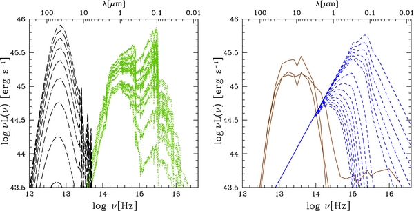
Figure 1. Examples of templates employed in the SED fitting code. Left panel: the black long-dashed and the green dotted lines correspond to the starburst and host galaxy templates, respectively. Right panel: the brown solid and blue dashed lines correspond to the hot dust from reprocessed AGN emission and BBB templates with increasing reddening, respectively.
Download figure:
Standard image High-resolution imageThe nuclear hot dust SED templates are taken from Silva et al. (2004). They were constructed from a large sample of Seyfert galaxies selected from the literature for which clear signatures of non-stellar nuclear emission were detected in the near-IR and mid-IR, and also using the radiative transfer code GRASIL (Silva et al. 1998). The infrared SEDs are divided into four intervals of absorption: NH < 1022 cm−2 for Seyfert 1, 1022 < NH < 1023 cm−2, 1023 < NH < 1024 cm−2, and NH > 1024 cm−2 for Seyfert 2. The latter case is neglected in our analysis. The three templates employed in the code are plotted in Figure 1 with the brown solid line. The NH estimates are used to select the torus template in the SED fitting code for each AGN in the sample. The mean NH of our sample is ∼1021 cm−2. Sixty-one percent (331/539) have NH consistent with no absorption, while the rest have a median of 7.5 × 1021 cm−2. A total of 446 objects (83%) have NH lower than 1022 cm−2; we have therefore considered the Seyfert 1 template for them. Only 17% (93/539) have NH greater than 1022 cm−2. For these sources dedicated templates (constructed considering Type 1 AGNs with NH > 1022 cm−2) are needed, but we have nevertheless employed the torus templates of Seyfert 2 for this sub-sample of sources. The Seyfert 1 torus template is not extremely different from the Seyfert 2 ones; hence, the results are not affected in any significant way.
We used a set of 30 galaxy templates built from the Bruzual & Charlot (2003, BC03 hereafter) code for spectral synthesis models, using solar metallicity and Chabrier initial mass function (Chabrier 2003). For the purposes of this analysis a set of galaxy templates representative of the entire galaxy population from passive to star forming is selected. To this aim, 10 exponentially decaying star formation histories (SFHs) with characteristic times ranging from τ = 0.1 to 10 Gyr and a model with constant star formation are included. For each SFH, a subsample of ages available in BC03 models is selected, to both avoid degeneracy among parameters and speed up the computation. In particular, early-type galaxies, characterized by a small amount of ongoing star formation, are represented by models with values of τ smaller than 1 Gyr and ages larger than 2 Gyr, whereas more actively star-forming galaxies are represented by models with longer values of τ and a wider range of ages from 0.1 to 10 Gyr. An additional constraint on the age is that, for each source, the age has to be smaller than the age of the universe at the redshift of the source. Each template is reddened according to the Calzetti et al. (2000) reddening law. The E(B − V)gal values range between 0 and 1 with a step of 0.05. A subsample of templates from star forming to passive (without reddening) is presented in Figure 1 (green dotted lines).
The BBB template representative of the accretion disk emission is taken from Richards et al. (2006). The near-infrared bump is neglected since we have already covered the mid-infrared region of the SED with the hot dust templates. This template is reddened according to the Prevot et al. (1984) reddening law for the Small Magellanic Clouds (SMC, which seems to be appropriate for Type 1 AGNs; Hopkins et al. 2004; Salvato et al. 2009). The E(B − V)qso values range between 0 and 1 with a variable step (ΔE(B − V)qso = 0.01 for E(B − V)qso between 0 and 0.1, and ΔE(B − V)qso = 0.05 for E(B − V)qso between 0.1 and 1) for a total of 29 templates. A subsample of templates with different reddening levels is presented in Figure 1 (blue dashed lines).
Figure 2 shows the distribution of the best-fit E(B − V)qso for our AGN sample from SED fitting. More than half of the sample is well fitted with low E(B − V)qso values (75% with E(B − V)qso ⩽ 0.1, 402 objects), with a median E(B − V)qso of 0.03. However, 137 Type 1 AGNs (24% of the total sample, 59 objects from the photo-z sample and 78 from the spectro-z sample) show evidence for a significant amount of obscuration11 (E(B − V)qso > 0.1). The fraction of photo-z Type 1 AGNs with E(B − V)qso > 0.1 is higher (43%, 59/136) than in the spectro-z sample (19%, 78/403). Given that the AGNs in the photo-z sample are, on average, fainter in the optical bands than those in the spectro-z sample, it is not surprising that the Type 1 AGNs in the photo-z sample have relatively higher reddening values than the spectroscopic Type 1s AGNs. In any case, the total fraction of reddened Type 1 AGNs in our sample is consistent with previous work in the literature (e.g., Richards et al. 2003; Maddox & Hewett 2006; Glikman et al. 2007).
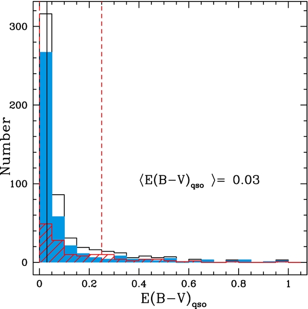
Figure 2. Disk reddening distribution for the main sample (open histogram). The spectro-z (cyan filled histogram) and photo-z (red hatched histogram) samples are also plotted. The solid line represents the median at 0.03, while the dashed lines correspond to the 16th and the 84th percentile at 0 and 0.25, respectively.
Download figure:
Standard image High-resolution imageIn Figure 3 the broad band SEDs of eight XMM-Newton Type 1 AGNs are plotted as examples. The four components adopted in the SED fitting code (starburst, AGN torus, host galaxy, and BBB templates) are also plotted. The red line represents the best fit, while the black points represent the photometric data used in the code, from low to high frequency: Herschel/MIPS-Spitzer (160 μm, 100 μm, 70 μm, and 24 μm if available), four IRAC bands, near-IR bands (J, H, and K), optical Subaru, CFHT, and GALEX bands. XID 9 and 126 are representative of a full SED with all detections from the far-infrared to the optical. Unfortunately, there are a limited number of detections at 160 and 70 μm (see Section 2.1), so that the more representative situation is shown in the other panels. XID 11 is representative of an AGN SED with contribution from the host galaxy in the near-IR, while for XID 146 and 51 the host galaxy contribution is almost negligible. XID 153, 13, and 69 represent cases where the host galaxy emission is significant. Subtracting the host galaxy contributions, especially for those sources with high stellar contamination, is therefore essential in order to measure, for example, the R parameter properly.

Figure 3. Examples of SED decompositions in the rest-frame plane. Black circles are the observed photometry in the rest frame (from the far-infrared to the optical–UV). The black long-dashed, brown solid, green dotted, and blue dashed lines correspond to the starburst, hot dust from reprocessed AGN emission, host galaxy, and BBB templates found as the best-fit solution, respectively. The red line represents the best-fit SED. XID, bolometric, and torus luminosities in erg s−1 are also reported.
Download figure:
Standard image High-resolution imageThe observed data points from infrared to optical are fitted employing a standard χ2 minimization procedure
where Fobs, i and σi are the monochromatic observed flux and its error in the band i; FSB, i, Ftorus, i, Fgal, i, and FBBB, i are the monochromatic template fluxes for the starburst, the torus, the host galaxy, and the BBB component, respectively; and A, B, C, and D are the normalization constants for the starburst, the torus, the host galaxy, and the BBB component, respectively. The starburst component is used only when the source has a detection between 160 μm and 24 μm. Otherwise, a three-component SED fit is used. Twenty is the maximum number of bands adopted in the SED fitting (only detections are considered), namely, 160 μm, 100 μm, 70 μm, 24 μm, 8.0 μm, 5.8 μm, 4.5 μm, 3.6 μm, KS, J, H, z+, i*, r+, g+, VJ, BJ, u*, NUV, and FUV.
For each source the code computes several physical parameters such as star formation rate (from both optical and far-infrared), stellar mass and colors of the host galaxy, AGN luminosity computed in different regions of the SED, and far-infrared luminosity of the cold dust. All outputs are estimated from the best-fit solution. The upper and the lower confidence levels of the luminosities are evaluated from the distribution of the normalizations of all fit solutions corresponding to 68% confidence level by taking the Δχ2 for a single parameter of interest (Δχ2 = 1; see Avni 1976). Large uncertainties on output parameters reflect the degeneracy among the templates involved in the fit, especially between star-forming galaxies and reddened BBB templates (see Figure 1).
4. ANALYSIS
In this section we discuss the computation of the mid-infrared to bolometric luminosity ratio, R, and the assumptions underlying its definition. We then present luminosities from both observed rest-frame SEDs and model fitting. Finally, we compare the luminosities computed with these two methods to highlight the impact of host galaxy and reddening correction on these measurements.
4.1. Mid-infrared to Bolometric Luminosity Ratio
The mid-infrared to bolometric luminosity ratio, which we employ to parameterize the obscured fraction, is defined as
where Ltorus is the infrared emission reprocessed by the dust at the wavelength range 1–1000 μm, while Lbol is our definition of the bolometric luminosity, which represents the optical–UV and X-ray emission emitted by the nucleus and reprocessed by the dust grains in the torus. There is some ambiguity in the literature about whether the X-ray emission, which partially arises from the accretion disk itself, but also from accretion disk photons Compton up-scattered by a hot X-ray corona, should be included in the bolometric luminosity. However, because we are here interested in all emission being reprocessed by dust grains, we include the X-ray contribution (∼10%) to the bolometric luminosity.12 Thus, we need to quantify the maximum frequency, νmax, which we define to be the frequency at which the dust optical depth in the torus, τd = Ndσd(ν), is unity, where Nd is the column density of dust in the torus and σd(ν) is the dust cross section. Photons with a frequency higher than νmax should not be counted in the bolometric emission budget, as they will just pass through the torus without being reprocessed.
Draine (2003b) estimated the X-ray extinction and scattering cross section per H nucleon due to interstellar dust, assumed to be a mixture of carbonaceous and amorphous silicate grains, and absorption due to gas with interstellar gas-phase abundances in the energy range 0.1–10 keV (see their Figure 6). Absorption by H and He dominates at energies lower than ∼0.25 keV, while above this energy value observations of extinction and scattering by dust are significant for bright sources with sufficient dust column densities along the line of sight. At E ⩾ 0.8 keV extinction is mainly due to dust grains. The energy at which the dust optical depth is equal to 1 considering an average NH value for obscured AGNs of ∼1022 cm−2 (see L12) is around 1 keV, which corresponds to a frequency of 2.4 × 10¹⁷ Hz. We have to integrate Equation (2) out to energies that are intercepted by the torus (not along our line of sight), and thus the average NH for Type 2 AGNs should be more appropriate. The precise energy of the absorption in the X-rays will be dependent on the chemical nature of the grain material (Forrey et al. 1998; Draine 2003a, 2003b); given that soft X-ray emission usually contributes about 10% of the total bolometric output, the uncertainty in our luminosity estimates due to the unknown X-ray opacity will be less than this. In order to quantify the degree of variation on the Lbol estimates, we have also considered an energy cutoff of 0.4 keV and 2 keV (frequency of 1017 and 4.8 × 10¹⁷ Hz), which correspond to an NH of about 1021 (the average value of the present Type 1 AGN sample) and 1.6 × 1022 cm−2, respectively.13 The shift induced by considering the difference between Lbol estimated up to a maximum energy cutoff of 0.4 and 2 keV is 〈ΔlogLbol〉 = −0.066 ± 0.004. Thus, our assumption of a 1 keV cutoff will result in uncertainties smaller than this, and this effect is much smaller than other uncertainties in our calculation, i.e., degeneracies between templates, uncertainties on the data, etc. We consider as our fiducial νmax value the frequency corresponding to the energy at 1 keV.
We can compute total luminosities in a given range in two ways, one by integrating the actual photometry, and the other by integrating the resulting best-fit SEDs output from the SED fitting code. For the first approach, no attempt is made to subtract off the host galaxy contribution or to de-redden the photometry (i.e., the BBB). For the latter approach, we present two cases. In the first case we have estimated R considering Lbol without correcting for the intrinsic AGN reddening. This approach is what has been used by other works on SEDs that tried to estimate covering fractions (see Maiolino et al. 2007; Treister et al. 2008). In the second case Lbol is corrected for both host galaxy and reddening contributions. In the next sections we will present these two ways of computing the total luminosities in a given range, and we will dedicate a separate discussion about the effect of the AGN reddening and host galaxy correction on Lbol.
4.2. Luminosities from Observed Rest-frame SED
We have computed the individual observed rest-frame SEDs for all sources in the sample, following the same approach as in L10. For the estimate of the rest-frame AGN SED we need to extrapolate the UV data to X-ray "gap" and at high X-ray energies. The SED is extrapolated up to 1200 Å with the slope computed considering the last two rest-frame optical data points at the highest frequency in each SED (only when the last UV rest-frame data point is at λ > 1200 Å). Then, a power-law spectrum to 500 Å is assumed, as measured by HST observations for radio-quiet AGNs (fν∝ν−1.8; see Zheng et al. 1997). The UV luminosity at 500 Å is then linearly connected (in the log space) to the luminosity corresponding to the frequency of 1 keV. We note that the fraction of bolometric luminosity in the 500 Å to 1 keV range depends on the model adopted, as shown by Krawczyk et al. (2013). However, these authors found that bolometric corrections estimated at 2500 Å, considering different UV–X-ray extrapolations, agree within a factor of about 1.5. Finally, the X-ray spectrum is extrapolated at higher energies, introducing an exponential cut off at 200 keV (e.g., Perola et al. 2002). An example of observed rest-frame SED is plotted in Figure 4 with the black dot–dashed line. We checked if the extrapolation works properly by inspecting all objects visually.
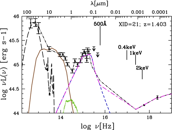
Figure 4. Example of full AGN SED from far-IR to X-rays at a redshift of 1.4 (XID = 21). The rest-frame data, used to construct the observed and fitted SEDs, are represented with black points. The black long-dashed, brown solid, green dotted, and blue dashed lines correspond to the best-fit starburst, hot dust from reprocessed AGN emission, host galaxy, and BBB templates, respectively. The black dot–dashed line represents the observed rest-frame SED as described in Section 4.2, while the magenta short–long dashed line is the best-fit BBB template plus X-rays as described in Section 4.3.
Download figure:
Standard image High-resolution imageObserved infrared and bolometric luminosities (hereafter LIR, obs and Lbol, obs) are quantified by integrating the observed rest-frame SED in the log space from 1 μm to 24 μm (Hao et al. 2012) and from 1 μm to 1 keV, respectively.
4.3. Luminosities from SED Fitting
The four-component SED fitting code presented here allows us to have a reliable estimate of both disk and torus luminosities (hereafter Ldisk and Ltorus). In Figure 4 a full AGN SED from far-infrared to X-rays, with the respective best-fits, is presented as an example. X-rays are not taken into account in the fit procedure. Therefore, in order to estimate Ldisk, we need to include them in a separate step. We consider the disk template up to 500 Å and the de-absorbed X-ray spectrum (as described in the previous section) at energies higher than 1 keV. We then linearly connect these two curves (an example is presented with the magenta short–long dashed line in Figure 4). The resulting disk+X-ray SED is integrated from 1 μm to 1 keV and is our definition of bolometric luminosity. Only 6 objects (2 spectro-z and 4 photo-z) out of 539 Type 1 AGNs do not require any disk component in the best fit. As a result, Ldisk is not available for these sources.14
The Ltorus values are computed by integrating the best-fit torus templates (brown solid line in Figure 4) from 1 to 1000 μm. Information on Ltorus is available from the best-fit models for 516 out of 539 (96%) Type 1 AGNs, but three of these sources have been removed because the optical–UV photometry is fitted with a galaxy template only (and therefore R cannot be estimated without constraints on Ldisk). This leads to a sub-sample of 513 Type 1 AGNs (388 spectro-z and 125 photo-z) with both Ltorus and Ldisk estimates.
For the remaining 19 Type 1 AGNs (4%) a torus template is not considered in the best fit. All of these sources are at high redshift (1.60 ⩽ z ⩽ 4.26). Three objects are detected at 24 μm, but the code is not considering the torus model in the best fit due to the combination of two facts: first, large error on the 24 μm detection, and second, IRAC and optical–UV photometry are nicely fitted with galaxy plus disk templates only. No photometric coverage in the mid-infrared is present for the other 16, which do not have a 24 μm detection.
As we have already pointed out, there are several factors that need to be taken into account when obtaining Lbol, obs by integrating the interpolated photometry. host galaxy emission and reddening are both present, and they can lead to over/underestimating AGN emission, respectively. The analysis presented here takes into account these contributions, thanks to our model fitting procedure, and we will discuss their effects on Lbol, obs in the following.
4.4. Disk Luminosities: Effect of the Host Galaxy and Reddening
Our first step in determining the intrinsic bolometric AGN emission is to subtract the host galaxy contribution from total observed Lbol without taking into account the AGN reddening. A comparison between Lbol, obs (from interpolated photometry) and Lbol (from model fitting, host galaxy subtracted) is presented in the left panel of Figure 5, where the one-to-one correlation is plotted with the red solid line as reference. The median shift between Lbol, obs, which includes both host galaxy and reddening contamination, and Lbol is 0.25 dex. Sources that deviate more from the average logLbol, obs/Lbol are those with higher host galaxy contamination and reddening. Twenty AGN (12 spectro-z and 8 photo-z) lie more than 3σ away from the median and are marked with orange open squares in Figure 5 (left panel). Representative examples of SEDs of these outliers are discussed in Appendix B. Part of the scatter and the fact that none of the sources lie on the one-to-one correlation might be due to the different methods of extrapolation in the UV–soft-X-ray gap (15.5 ≲ logν ≲ 17.5 Hz) adopted (see Figure 4). In order to check this issue, we have estimated, for each object, the observed optical–UV luminosity (Lopt-UV, obs) by integrating the interpolated rest-frame photometry between 1 μm and the bluest rest-frame data point in the optical–UV, and the fitted optical–UV luminosity (Lopt-UV) by integrating the best-fit BBB template in the same wavelength range. The result is plotted in the right panel of Figure 5. Sources are now closer to the one-to-one relation (with 16 outliers), but the scatter is still significant, demonstrating that the host galaxy contribution is important in the optical–UV.
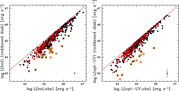
Figure 5. Left panel: comparison between the values of Lbol computed by the SED fitting code (host galaxy subtracted) and those obtained integrating the observed rest-frame SED from 1 μm to 1 keV (see Section 4.2). Reddening has not been taken into account in the Lbol values. 3σ outliers from the median are marked with orange open squares (20 objects). Black points and red triangles represent the spectro-z and photo-z samples, respectively. The red solid line represents the one-to-one correlation. The average error on Lbol is plotted in the bottom right for clarity. Right panel: comparison of the observed optical–UV luminosity (Lopt-UV, obs) by integrating the interpolated rest-frame photometry between 1 μm and the bluest rest-frame data point in the optical–UV with the fitted optical–UV luminosity (Lopt-UV) by integrating the best-fit BBB template in the same wavelength range (16 outliers, open orange squares).
Download figure:
Standard image High-resolution imageWe have also computed the host galaxy luminosity (Lhost) from the best-fit galaxy template for each Type 1 AGN over the same wavelength range of Lopt-UV. For a significant fraction of the objects Lhost is comparable to Lopt-UV. For example, we found that the ratio between Lhost and Lopt-UV is more than 0.7 for 34% of the Type 1 AGNs in our sample.
Overall, our model fitting procedure highlights a significant host galaxy contamination in the bolometric emission of Type 1 AGNs in XMM-COSMOS, in agreement with previous results (see also Figure 4 in Bongiorno et al. 2012). In a recent paper (Elvis et al. 2012) the average SED of the same COSMOS sample employed here is presented. It is clear from Figure 14 in Elvis et al. (2012) that the mean observed SED is quite flat and lacks the 1 μm inflection point between the UV and near-IR bumps seen in previous analyses. This suggests that this sample has a higher contamination from the host galaxy light than brighter optically selected samples (see Elvis et al. 2012; Hao et al. 2012).
The next step in determining the intrinsic nuclear Lbol is to correct for reddening the best-fit BBB template by employing the corresponding E(B − V)qso value for each object in our sample. The reddening-corrected best-fit bolometric luminosities are plotted in the left panel of Figure 6 as a function of Lbol, obs. As expected, AGNs with high E(B − V)qso tend to have higher Lbol than Lbol, obs, with the ratio of the corrected Lbol and Lbol, obs distributed almost symmetrically around zero (see right panel of Figure 6), but with a tail toward small values resulting from highly reddened systems. Outliers deviating more than 3σ below the median (two objects, which are superimposed in the plot) represent high host galaxy contamination, while outliers deviating more than 3σ above the median (nine objects) have large values of E(B − V)qso (E(B − V)qso ∼ 1) and small contribution from the host galaxy. Representative SEDs of these outliers are presented in Appendix C.
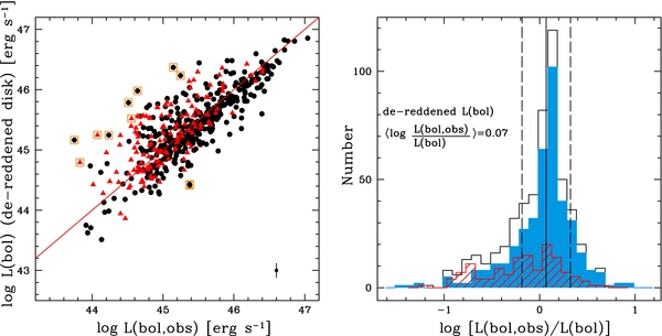
Figure 6. Left panel: comparison between the values of Lbol computed by the SED fitting code (see Section 4.3) and those obtained integrating the observed rest-frame SED from 1 μm to 1 keV (see Section 4.2). Reddening has been taken into account in the Lbol values. Black points and red triangles represent the spectro-z and photo-z samples, respectively. The red solid line represents the one-to-one correlation, while 3σ outliers are marked with orange open squares. Right panel: histogram of the ratio between Lbol, obs and Lbol. Key as in Figure 2. The solid line represents the median at logLbol, obs/Lbol = 0.07, while the dashed lines correspond to the median absolute dispersion (1.4826 × MAD; see Section 5) at 0.25 dex.
Download figure:
Standard image High-resolution imageAs a further check we have compared the infrared luminosities estimated from the observed rest-frame SED and those output from our SED fitting code. The left panel of Figure 7 shows this comparison. The majority of the sources lie along the one-to-one correlation with a median shift between the observed infrared luminosity and the torus luminosity of 〈logLIR, obs/Ltorus〉 = 0.10 (see the right panel of Figure 7), meaning that the infrared emission observed is mainly originated from hot dust. The tail at high logLIR, obs/Ltorus values is likely due to some contamination from star formation, which has been subtracted using the fitting technique. Outliers are again defined as those at more than 3σ away from the median. Six percent (32/513) of the sample and only two sources lie below and above 3σ from the median, respectively. Their SEDs are discussed in Appendix D.
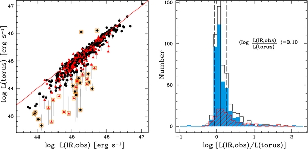
Figure 7. Left panel: comparison between the values of torus luminosity computed by the SED fitting code and those obtained integrating the observed rest-frame SED from 1 μm to 24 μm. Symbols are as in Figure 5. Gray bars represent 1σ error as discussed in Section 3. Right panel: histogram of the ratio between LIR, obs and Ltorus. Colors are as in Figure 2. The solid line represents the median at logLIR, obs/Ltorus = 0.10, while the dashed lines correspond to the median absolute dispersion (1.4826 × MAD; see Section 5) at 0.16 dex
Download figure:
Standard image High-resolution imageIn summary, AGN bolometric luminosities need to be corrected for the effects of both host galaxy contamination and intrinsic AGN reddening. Studies that do not take these factors into account may bias results on AGN obscuring fractions. To further emphasize this last point, in the following section we present a comparison of the R–Lbol relations under different assumptions: (1) the relation is presented without correcting for host galaxy and reddening, (2) considering Lbol and Ltorus from the model fitting where the Lbol values are host galaxy subtracted, and, finally, (3) where both effects of the host galaxy and reddening are considered.
5. MID-INFRARED TO BOLOMETRIC LUMINOSITY RATIO VERSUS Lbol
Previous analyses have found a decrease of the mid-infrared luminosity ratios as a function of bolometric (i.e., accretion disk) luminosity (see e.g., M07; Treister et al. 2008; Hatziminaoglou et al. 2009), which has been interpreted as a corresponding decrease in the obscured fraction with luminosity, but these previous works have one (or more) of the following limitations: (1) disk luminosities and/or mid-infrared luminosities have been estimated using uncertain bolometric corrections, (2) host galaxy light has not been subtracted out, and (3) the disk has not been de-reddened in computing the bolometric luminosity.
In Section 4.4, we have seen that reddening can lead one to significantly underestimate the true bolometric luminosity and hence the luminosity ratio R (the relation between the obscured fraction and R is discussed in Section 6). Figure 8 (panel (a)) shows our observed logLIR, obs/Lopt, obs values as a function of Lopt, obs, where green points are the median of logLIR, obs/Lopt, obs in each bin (defined to have approximately the same number of sources in each bin, about 77 objects). The luminosities have been determined by integrating the interpolated observed photometry (see Section 4.2), as has the observed bolometric luminosity plotted on the x-axis. The errors on these luminosities are negligible, and so we do not show estimates here. The bars on the y-axis represent the uncertainty on the median estimated as the standard deviation divided by the square root of the number of objects in each bin (σmed = 1.4826 × MAD/ ; Hampel 1974; Hoaglin et al. 1983; Rousseeuw & Croux 1993).15 The bars on the x-axes are the width of the bin. We decided to consider the median instead of the mean, because our measures are sometimes moderately disperse (e.g., Ltorus/Lbol as a function of Lbol in Figure 8). Mean and standard deviation are heavily influenced by extreme outliers. The median and the MAD provide a measure of the core data without being significantly affected by extreme data points. In order to further check that the MAD is actually a robust estimator of our distribution, we have compared MAD with both bootstrap analysis and percentile. All uncertainties are consistent among the three different methods. We have then considered only one method (i.e., MAD) throughout the paper for ease of discussion.
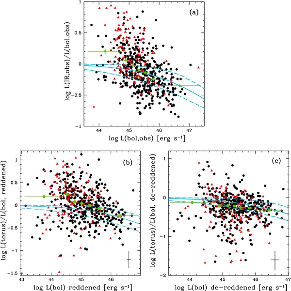
Figure 8. Panel (a): logLIR, obs/Lopt, obs as a function of Lopt, obs computed from the observed rest-frame SED. Black points and red triangles represent the spectro-z and photo-z samples, respectively. Green points are the median of the logLIR, obs/Lopt, obs values in each bin (about 77 sources per bin), the bars on the y-axis represent the uncertainty on the median, while the bars on the x-axis are the width of the bin. The cyan line shows the mid-infrared luminosity ratios inferred by M07. Dashed lines trace the uncertainties due to bolometric correction. Panel (b): logLtorus/Lbol as a function of host galaxy-corrected Lbol without reddening correction (about 73 sources per bin). Panel (c): logLtorus/Lbol as a function of Lbol with both host galaxy and reddening correction (about 73 sources per bin). The average uncertainties on Lbol and logLtorus/Lbol are plotted in the bottom right of panels (b) and (c).
Download figure:
Standard image High-resolution imageM07 present mid-infrared luminosity ratios for a sample of 25 high-luminousity QSOs at redshift 2 < z < 3.5 with Spitzer-IRS low-resolution mid-IR spectra, combined with data for low-luminosity Type-1 AGNs from archival IRS observations. Their definition of obscuring fraction is based on the luminosity ratio at 6.7 μm and 5100 Å, corrected by a fixed kbol (f = 0.39 L6.7 μm/L5100 Å, where the thermal infrared bump is defined as 2.7 L6.7 μm and the accretion disk luminosity is 7 L5100 Å), and where the X-ray emission is neglected. To compare our results with M07, we have then converted their L5100 Å values using a kbol of 7. The variation of the obscuring fraction as a function of luminosity found by M07 is also plotted in Figure 8 with the solid cyan line, while the dashed lines represent the M07 estimate of the uncertainty due to their adopted bolometric correction. Our points in Figure 8(a) (ignoring host galaxy contamination and not de-reddening the disk) show a similar trend as the M07 relation. M07 has a flatter distribution, less affected by host galaxy contamination at low Lbol, while our measurements show a steeper decline with luminosity. This further emphasize that proper host galaxy and reddening correction is needed especially at low luminosities.
The M07 analysis assumes that the luminosity ratio is equivalent to the obscured AGN fraction (i.e., optically thin torus regime; see Section 6.3). Our median LIR, obs/Lbol, obs value is  . A Spearman rank test gives the correlation coefficient, ρ, of −0.51, excluding the null correlation at the level of about 14σ.
About 37% (199/539) have observed LIR, obs/Lbol, obs values higher than 1, which is not physical given our assumption on the optically thin torus (i.e., the energy has to be conserved). However, this could be due to several factors, such as uncertainties in the observational data (83 objects over 199 AGNs with LIR, obs/Lbol, obs > 1 do not have spectroscopic redshift measurement), reddening and/or host galaxy contamination, and non-trivial torus radiative transfer effects, i.e., optically thick torus.
The above discussion of Figure 8(a) regards the logLIR, obs/Lbol, obs–logLbol, obs relationship, where no host galaxy and AGN reddening correction has been performed. If we now use our SED fitting to take into account and effectively subtract off host galaxy contamination from the Lbol estimates, without correcting for AGN reddening, the overall effect is to shift R (defined as in Equation (2)) to higher values and move Lbol to lower luminosities as shown in Figure 8 (panel (b)). This is because host galaxy light more significantly contaminates the near-IR to UV part of the SED than it does in the mid-infrared, and hence it significantly impacts our Lbol estimates. This is especially true for those cases where the optical–UV region is fitted with a star-forming galaxy template (i.e., XID = 16, 2072, and 53583 in Figure 21), which would lead to unphysical results. In fact, on average the R values determined from SED fits and where the host galaxy is subtracted are only a factor of ∼1.2 higher than the R determined from integrated photometry, with a median R of  (ρ = −0.33, excluding the null correlation at the level of about 8σ). The shift to higher R values is mainly due to the employed Lbol, given that the observed and the fitted torus luminosities are quite similar16 (except outliers discussed in Appendix D). The resulting trend between R and Lbol is still present, although with a different normalization.
Each best-fit BBB template has then been de-reddened considering the corresponding E(B − V)qso output of the SED fit. Figure 8 (panel (c)) shows the R values as a function of Lbol after employing this correction. The median R is  (ρ = −0.19, excluding the null correlation at the level of about 4σ). About 19% (99/513) still have R factors higher than 1 (70 spectro-z and 29 photo-z). The SEDs of these objects have, on average, a high host galaxy contamination at low Lbol (four examples are presented in Figure 9).
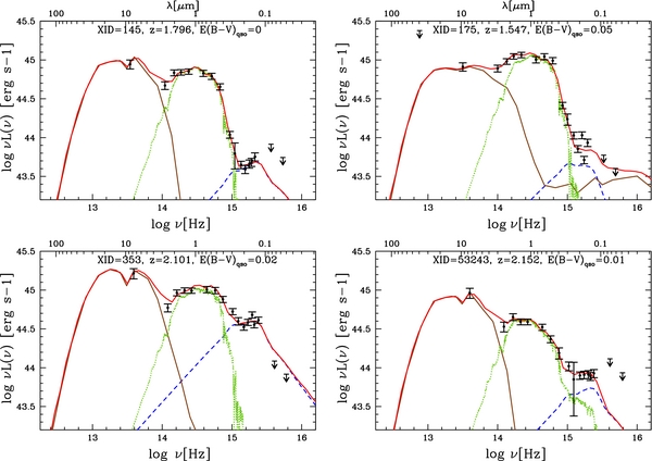
Figure 9. Example of SEDs with R > 1. Line types and colors are as in Figure 3.
Download figure:
Standard image High-resolution imageSummarizing, we find that the average observed R value for the Type 1 AGN sample presented here is 0.81, with a clear trend of decreasing R with increasing Lbol, obs. We still observe the same trend between R and Lbol if we compute R from the output luminosities of our SED fitting code, and correcting for the host galaxy contribution only, but the average R is higher than the observed one (〈R〉 ≃ 0.98). We therefore need to consider the effect of the intrinsic AGN reddening as well, whose correction leads to a more reasonable value of R (〈R〉 ≃ 0.57), while our relation between R and Lbol is shallower than in earlier works (e.g., M07). This is presumably because, differently from previous analyses, we have corrected for dust reddening and subtracted off the host. Therefore, the correct average R value is the one taking into account both corrections (i.e., 〈R〉 ≃ 0.57).
We conclude that any SED-based analysis needs to take into account the intrinsic AGN reddening/host galaxy contamination in order to properly estimate R and its variation on luminosity. Throughout the following discussion, we consider the intrinsic Lbol the one reddened corrected and where the host galaxy has been subtracted.
6. DISCUSSION
6.1. AGN Obscured Fraction: Optically Thin versus Optically Thick Tori
The infrared emission detected by an observer along a line of sight that crosses the torus (Type 2) might differ from the one along a dust-free sightline (Type 1), which is to say that infrared emission from the torus could be anisotropic. Following Granato & Danese (1994, GD94 hereafter), we define the ratio between the integrated flux emitted by the dust in the direction of the equator and that emitted in the direction of the pole as p (see their Equation (22)). This parameter, which quantifies the anisotropy of the radiation emitted by the torus, is directly related to the obscured fraction fobsc, and it depends on the optical depth (at a fixed fobsc and for a given geometry; see GD94 Figure 10) of the torus to its own mid-infrared radiation. The basic idea is that if we assume that the bulk of the infrared radiation is produced by an optically thick (to its own infrared radiation) dusty torus, and the observer has an absorption-free line of sight, fobsc is related to the R (R = Ltorus/Lbol) and p factors as follows:
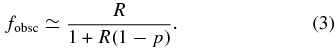
For a torus transparent to its own radiation (optically thin) the parameter p is of the order of unity (no viewing angle dependence), and therefore fobsc ∼ R. If the torus is instead optically thick, the torus behaves like a blackbody, and the obscured fraction, for a given value of R, is lower than the one in the optically thin regime.
GD94 studied a sample of 56 local (z ⩽ 0.08) optically selected radio-quiet Seyferts, of which 16 are unobscured (Seyfert 1). In the case of unobscured AGNs, GD94 find that the observed infrared continuum originates from an almost homogenous dust distribution, extending at least a few hundred parsecs, with fobsc ⩽ 0.6. The GD94 radiative transfer models also show that optically thick and broad (extending for ∼1000 pc at optical luminosities of the order of 1046 erg s−1; but see also Tristram & Schartmann 2011) tori are able to explain the infrared continua observed in both Type 1 and Type 2 AGNs.
Nenkova et al. (2008b) considered clumpy torus models and showed that a total of 5–15 optically thick dusty clouds along the radial equatorial line of sight can successfully explain AGN infrared observations. Further observational evidence from interferometry (e.g., Kishimoto et al. 2007) and molecular emission lines (e.g., Pérez-Beaupuits et al. 2011) favors a clumpy, rather than smooth, dust distribution in AGN tori. This has stimulated additional modeling efforts by several authors (e.g., Dullemond & van Bemmel 2005; Hönig & Kishimoto 2010, and references therein). Interestingly, another set of simulations of clumpy torus models by Hönig & Kishimoto (2011) have found that, although the clouds are optically thick, the observed SED is dominated by emission from optically thin dust in Type 1 AGNs.
Given all the conflicting views about whether the torus is optically thick or thin to infrared radiation, we remain agnostic and consider p as a free parameter. But in order to compute fobsc, we would need a determination of p for each source in our sample, which would require information about the mid-infrared optical depth of each AGN's torus. Since such estimates are not available and, moreover, as p strongly depends on assumptions about the distribution of dust in the torus and its geometry, we instead explore the two extreme cases where p = 1 (fobsc = R, optically thin torus) and p ≪ 1 (fobsc ≃ R/(1 + R), optically thick torus). The true obscured AGN fraction is bounded by these two extremes.
6.2. Dust-reddened AGN Population
All of our analysis on the obscured fraction is based on the parameter R, which is the ratio between the mid-infrared and the bolometric emission. In the presence of a reddened optical–UV emission, our model fitting procedure should be able to correct for the extinction, so that we can use the de-reddened Lbol. However, as we have mentioned at the beginning of this section, the infrared emission along a line of sight that crosses the torus can be different from the one along a dust-free line of sight, and this difference increases as the torus becomes more optically thick (p decreases from unity). The difference goes in the direction that infrared emission from an obscured line of sight (i.e., equatorial emission) is smaller than along a non-obscured line of sight (i.e., polar emission). In cases for which we find that our Type 1 BBB disk model fits require significant extinction, these lines of sight are not strictly speaking dust-free, and their (more equatorial) infrared emission will tend to be smaller. However, the application of Equation (3) from GD94 requires that the Ltorus in the numerator of R is determined from a (more polar) dust-free line of sight, i.e., it is the Ltorus of a Type 1 AGN. Thus, highly extinct Type 1 AGNs will have smaller Ltorus values, resulting in lower values for R, and thus the obscured fraction that we obtain for such objects would be systematically smaller than it is in reality.
Such highly reddened AGNs, which are broad-line sources with nevertheless significantly reddened BBB SEDs, clearly reside in a gray area of the AGN unification classification into only two types of AGN (i.e., purely obscured and unobscured). These sources are likely observed from intermediate viewing angles, and thus the simple modeling of GD94 (parameterized by a Type 1 AGN polar Ltorus emission) is no longer applicable for such objects. We thus quantify the fraction of such reddened AGNs in our sample by considering the best-fit E(B − V)qso output of our model fitting (see Figure 2).
In what follows, we present our results for the main sample of 513 Type 1 AGNs and for the sub-sample of 391 objects with E(B − V)qso ⩽ 0.1. Our choice of E(B − V)qso = 0.1 is rather arbitrary, but it is effective in defining a sub-sample of AGNs with representative SEDs of the main population (see Figure 2, but see also Figure 6 and related discussion in Richards et al. 2003).
6.3. Dependence of Obscured AGN Fraction on Bolometric Luminosity
Our estimates of the obscured AGN fraction as a function of Lbol in the optically thin and optically thick regimes described above are presented in Figure 10. Filled circles represent the optically thin torus case, while open circles show the results for the thick torus prescription. As a comparison, we have overplotted fobsc as found by M07. For completeness we also plotted the mean fobsc in each bin and the 1σ error bars. The mean fobsc of the first bin is out of scale (i.e., 〈fobsc〉 = 1.24). Mean fobsc estimates are more sensitive to the data with fobsc > 1 (20% of the all sample, but mainly found at the low-luminosity end); thus, in this case the median is more representative of our obscuring fraction distribution. By defining the obscured fraction fobsc = R, the M07 analysis assumes an optically thin torus (solid cyan line in Figure 10). If we instead consider the optically thick case where p ≪ 1, the obscured AGN fraction implied by the M07 R measurements is reduced as shown by the dot–dashed cyan line. We confirm that a decrease of fobsc with increasing Lbol exists in both the main sample (left panel of Figure 10) and the sample with E(B − V)qso ⩽ 0.1 (right panel of Figure 10). Our fobsc − Lbol relations are within M07's 1σ dispersion. Assuming the optically thin case, the obscured AGN fraction for the main sample changes from ∼75% at Lbol ≃ 1.5 × 1044 erg s−1 to ∼45% at Lbol ≃ 2.5 × 1046 erg s−1. This decreasing trend is strongly suppressed in the optically thick torus regime, where fobsc ranges approximately from ∼45% to ∼30%. If we instead consider the low-reddening sub-sample, the slope of the fobsc–Lbol relation does not change significantly, but the normalization is shifted to higher fobsc values. This is expected because the full sample includes the reddened AGNs, which tend to have lower Ltorus (see Section 6.2) and hence lower R values, implying lower obscured fractions.
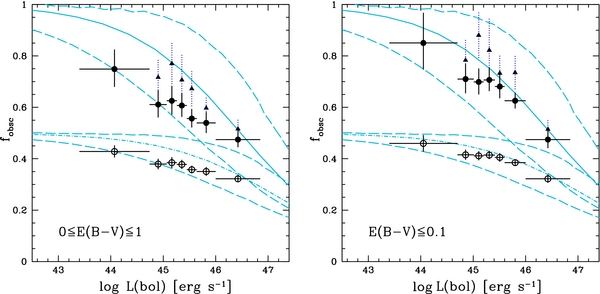
Figure 10. Left panel: obscured AGN fraction as a function of Lbol for the main sample of 513 Type 1 AGNs. Filled circles represent our median estimates of the fobsc parameter in the optically thin torus regime (p = 1), while open circles represent the fobsc parameter in the optically thick torus regime (p ≪ 1). Triangles represent the mean of the obscuring fraction in each bin, while dotted lines are 1σ error bars. The cyan solid line is the obscured AGN fraction as originally estimated by M07 (thin case), while the cyan dot–dashed line represents the obscured AGN fraction by M07 in the optically thick torus case. Dashed lines trace the uncertainties due to bolometric correction. Right panel: obscured AGN fraction as a function of Lbol for the 391 Type 1 AGNs with E(B − V)qso ⩽ 0.1.
Download figure:
Standard image High-resolution imageAnother SED-based approach has been presented in Treister et al. (2008, T08 hereafter). This analysis considers 230 Type 1 AGNs (with spectroscopic redshifts) at z ∼ 1, selected from several surveys (206 AGNs are drawn from SDSS, 10 from GOODS, and 14 from COSMOS), with archival 24 μm MIPS photometry, and GALEX data. This sample spans a similar range in Lbol from 1044 to 1047.5 erg s−1, and their fobsc measurements are plotted in Figure 11 with gray open squares. T08 argue that their measurements agree with M07, and the agreement is rather remarkable; however, in the T08 analysis fobsc is estimated by assuming an anisotropic infrared emission coming from an optically thick torus (p ≪ 1; see their Equation (1)), whereas the M07 results are derived under the assumption of an optically thin torus fobsc ∼ R. The level of agreement between fobsc by M07 and those evaluated by T08 is therefore unexpected. The obscured fraction produced by an optically thick torus should be lower than the one originated in a thin torus at a given R = Ltorus/Lbol ratio.

Figure 11. Obscured AGN fraction as a function of Lbol in the optically thick torus regime (p ≪ 1) for the 391 Type 1 AGNs with E(B − V)qso ⩽ 0.1. Open circles represent our estimates of the fobsc parameter. Open squares are the fobsc estimates by T08 (thick regime).
Download figure:
Standard image High-resolution imageIn order to understand this rather confusing agreement between T08 and M07, it is worth discussing the T08 analysis in more detail. The obscured AGN fraction in T08 is evaluated from the ratio between the observed luminosity at 24 μm, corresponding approximately to the rest-frame 12 μm luminosity, and the bolometric luminosity (neglecting X-ray emission), and with no correction for host galaxy and reddening contamination. Consequently, they need to compute the fraction of the total dust-reprocessed luminosity falling within the MIPS band as a function of opening angle (f12(θ)), which can be interpreted as the inverse of a bolometric correction in the infrared. They find that f12(θ) varies from 0.06 to 0.08 considering a series of models constructed with the code described in Dullemond & van Bemmel (2005). These f12(θ) values correspond to a bolometric correction at 24 μm of ∼12.5–17, which might be responsible for higher total mid-infrared luminosity than the one we observed, and therefore leading T08 to overestimate the obscured fraction. However, we note that a bolometric correction of 10 (consistent with the recent findings by Runnoe et al. 2012) does not lead to a significantly better agreement with the optically thick case. Given the angular dependence of f12(θ), it is not straightforward to determine what aspect of the T08 calculation leads to overestimated obscured fractions. We have also estimated the obscuring fraction for a sub-sample of AGNs in the same redshift range explored by T08 (0.8 ⩽ z ⩽ 1.2, 89 objects with 0 ⩽ E(B − V)qso ⩽ 1, 70 with E(B − V)qso ⩽ 0.1), but we do not find a better agreement. However, we caution that this sub-sample is significantly smaller than the one considered by T08.
The agreement between M07 and T08 thus remains puzzling, given that our analysis is consistent with M07 under similar assumptions and has been carried out with a completely independent method and without any bolometric correction prescription.
6.4. Comparison to Demographic-based Analysis
We can now compare our fobsc estimates with demography-based analyses (e.g., Hao et al. 2005; Simpson 2005, hereafter S05). S05 used a magnitude-limited AGN sample17 from SDSS to determine that the fraction of Type 2 AGNs relative to the total (i.e., the obscured fraction) decreases with the luminosity of the [O iii] narrow emission line, where it has been assumed that the [O iii] luminosity is a good proxy for the bolometric AGN emission and, crucially, that the Type 2 AGN sample is complete.
A comparison of our measurement of the obscured AGN fraction with that of S05 is presented in Figure 12 for the total and the low-reddening AGN sample. We converted the [O iii] luminosities to bolometric using kbol of ∼3200 (Shen et al. 2011). We find that the obscured fraction estimated by S05 is fully consistent with the optically thin torus regime. Given that the fobsc values from S05 are computed using a completely different and independent method, this may be an indication that the reprocessed infrared emission in AGNs occurs in the optically thin regime (we will address this issue in Section 6.7). Assuming a constant ![$k_{{[\rm {O\,\scriptsize{III}}]}}$](https://content.cld.iop.org/journals/0004-637X/777/2/86/revision1/apj485146ieqn9.gif) for
for ![$L_{{[\rm {O\,\scriptsize{III}}]}}$](https://content.cld.iop.org/journals/0004-637X/777/2/86/revision1/apj485146ieqn10.gif) is a rather crude approximation, as it has been found that an anti-correlation exists between the equivalent widths of emission lines and the continuum luminosity of AGNs, i.e., the so-called Baldwin effect, may also exist in narrow emission lines such as [O iii] (e.g., Dietrich et al. 2002; Netzer et al. 2004; Zhang et al. 2013; but see also Croom et al. 2002 for a different result). If the [O iii] luminosity can be considered a good proxy for Lbol (e.g., Heckman et al. 2004), there may be the possibility that the
is a rather crude approximation, as it has been found that an anti-correlation exists between the equivalent widths of emission lines and the continuum luminosity of AGNs, i.e., the so-called Baldwin effect, may also exist in narrow emission lines such as [O iii] (e.g., Dietrich et al. 2002; Netzer et al. 2004; Zhang et al. 2013; but see also Croom et al. 2002 for a different result). If the [O iii] luminosity can be considered a good proxy for Lbol (e.g., Heckman et al. 2004), there may be the possibility that the ![$k_{{[\rm {O\,\scriptsize{III}}]}}$](https://content.cld.iop.org/journals/0004-637X/777/2/86/revision1/apj485146ieqn11.gif) value is very different from what we have considered and may not be constant with Lbol. We have then applied the relation between Lbol and [O iii] luminosity as found recently by Stern & Laor (2012, see their Equation (4)), and the data are still fully consistent with an optically thin torus.
value is very different from what we have considered and may not be constant with Lbol. We have then applied the relation between Lbol and [O iii] luminosity as found recently by Stern & Laor (2012, see their Equation (4)), and the data are still fully consistent with an optically thin torus.
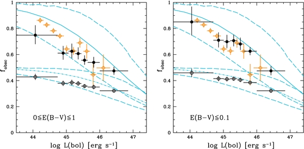
Figure 12. Left panel: obscured AGN fraction as a function of Lbol for the main sample of 513 Type 1 AGNs. Filled circles represent our median estimates of the fobsc parameter in the optically thin torus regime (p = 1), while open circles represent the fobsc parameter in the optically thick torus regime (p ≪ 1). The cyan solid line is the obscured AGN fraction as originally estimated by M07 (thin case), while the cyan dot–dashed line represents the obscured AGN fraction by M07 in the optically thick torus case. Dashed lines trace the uncertainties due to bolometric correction. Right panel: obscured AGN fraction as a function of Lbol for the 391 Type 1 AGNs with E(B − V)qso ⩽ 0.1. Open diamonds are the fobsc values estimated by S05.
Download figure:
Standard image High-resolution imageReyes et al. (2008) present the obscured AGN fraction (i.e., the ratio of Type 2 to total (Type 1 + Type 2) quasar number densities) for a large sample of optically selected Type 2 AGNs from SDSS with redshifts z < 0.83. They carefully take into account selection effects and biases in their estimate of the obscured fraction, giving reliable lower limits to this parameter (in agreement with S05 results). In their analysis it is clearly pointed out that [O iii] luminosity is not a perfect tracer of Lbol, and there is considerable scatter between these two luminosities for Type 1 AGNs (see their Figure 9; see also Netzer et al. 2006 for similar results). They have also found indications that the [O iii] line is slightly more extincted in Type 2 AGN than in Type 1. These findings thus conclude that AGN samples selected through this line might be biased toward Type 1 objects, and this would artificially reduce the obscured AGN fraction derived in demography-based studies.
Summarizing, we confirm that a correlation exists between fobsc and the Lbol in the optically thin regime, while the correlation is very weak in the thick case. The slope of the fobsc–Lbol relation does not vary significantly considering the total and the low-reddening AGN sample, but the overall relation for the low-reddening AGN sample is shifted to higher fobsc than the one for the total AGN sample. Finally, a comparison of our SED-based obscured fraction results to demography-based determinations seems to favor the optically thin regime.
6.5. Dependence of Obscured AGN Fraction on Hard X-Ray Luminosity
Ueda et al. (2003) were the first to find a significant (almost linear) decrease of the obscured AGN fraction with increasing hard X-ray luminosity (L[2–10] keV; see also Steffen et al. 2003), considering a combination of hard X-ray surveys, namely, the High Energy Astronomy Observatory 1 (HEAO 1), ASCA, and Chandra for a total of 247 AGNs in the 2–10 keV luminosity range of 1041.6–46.5 erg s−1 and redshift up to 3. After that work, a series of almost independent analyses of X-ray-selected samples have been performed confirming this trend (e.g., Steffen et al. 2003; Barger et al. 2005; La Franca et al. 2005; Hasinger 2008). All these works have computed the obscured AGN fraction considering the ratio of Type 2 AGNs over the total AGN population.
Figure 13 shows the obscured fraction as a function of L[2–10] keV in the optically thin (p = 1, filled circles) and thick (p ≪ 1, open squares) regime for the main sample (0 ⩽ E(B − V)qso ⩽ 1, top row), and for the low-reddening AGN one (E(B − V)qso ⩽ 0.1, bottom row). As a comparison, we have over plotted fobsc measurement from Ueda et al. (2003) (open squares), Hasinger (2008) (open triangles), and the fobsc − L[2–10] keV relation found by Treister et al. (2009, brown dashed curve, T09 hereafter), utilizing a demographic approach, for 339 X-ray AGNs in the Extended Chandra Deep Field South. There are several interesting points to note. First, we find that fobsc does not show a clear trend with L[2–10] keV, but it has a peak at ∼2 × 1044 erg s−1 and decreases toward low L[2–10] keV. Second, the variation of fobsc with L[2–10] keV in the optically thick regime is extremely weak. Third, X-ray demography-based samples find an obscured fraction lower than our estimates (SED-based) by a factor of ∼2 in the optically thin regime, and by a factor of ∼1.3 in the optically thick one at high L[2–10] keV (>1044 erg s−1). Evidence for a higher fobsc than X-ray surveys has already been obtained by Reyes et al. (2008). They find a lower limit of the obscured fraction significantly higher than that derived from X-ray surveys (especially Hasinger 2008 and T09) at [O iii] luminosities higher than 1043 erg s−1.
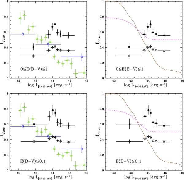
Figure 13. Top row: obscured AGN fraction as a function of the X-ray luminosity for the total AGN sample assuming p = 1 (filled black circles) and p ≪ 1 (open black circles), Ueda et al. (2003, blue open squares), and Hasinger (2008, green open triangles). The magenta dashed line represents the ratio of Compton-thin absorbed AGNs to all Compton-thin AGNs assumed in the Gilli et al. (2007) population synthesis model. The long-dashed brown line represents the fobsc–L[2–10] keV relation found by Treister et al. (2009). Bottom row: obscured AGN fraction as a function of the X-ray luminosity for the low-reddening AGN sample. Lines and symbols are as in the top row.
Download figure:
Standard image High-resolution imageOur SED-based obscured fraction determination provides an independent confirmation that X-ray demographic analyses are systematically missing obscured and highly obscured AGNs, which are likely to be the Compton thick AGNs.
In Figure 13 we also show the relation between absorbed (i.e., 21.5 < logNH [cm−2] < 23.5) Compton-thin AGNs and all Compton-thin AGNs assumed in the Gilli et al. (2007, G07 hereafter) X-ray background population synthesis model (a luminosity-dependent fobsc parameter has been assumed). The G07 model predicts a relatively large fraction of obscured AGNs, ∼50%, at high luminosities, while the observed value by T09 is only ∼20%. Our fobsc estimates show a different behavior in both the optically thick and thin regimes than the fobsc–L[2–10] keV relation in G07. However, at L[2–10] keV > 1044 erg s−1 the fobsc values we observe are in better agreement with the fobsc values in G07 if we consider the optically thin case.
While in Section 6.3 we observed an essentially monotonically linear decrease of fobsc with log Lbol, we find a non-monotonic dependence of fobsc on log L[2–10] keV and thus no compelling evidence for a decreasing trend with hard X-ray luminosity. The differing behavior of fobsc with these luminosities could be explained if Lbol and L[2–10] keV are not monotonically related, and/or if their relationship has a large scatter. In Figure 14 Lbol is plotted as a function of L[2–10] keV. The relation seems to be almost linear, although the scatter is large (∼0.44 dex).
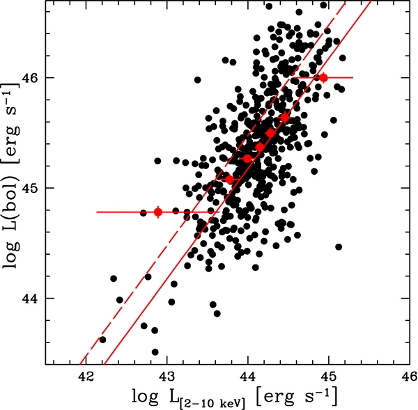
Figure 14. Bolometric luminosity as a function of L[2–10] keV. Red points are the median of the Lbol values in each bin (about 73 sources per bin), the bars on the y-axis represent the uncertainty on the median (1.4826 × MAD ; see Section 5), and the bars on the x-axis are the width of the bin. The red solid line represents an average hard X-ray bolometric correction of ∼15 (Lbol/L[2–10] keV; see Figure 9 in L12 for the average Lbol of our sample of ∼2.5 × 1045 erg s−1). The red dashed line represents Lbol/L[2–10] keV ∼ 30 (see Figure 3 in Marconi et al. 2004 for Lbol ∼ 2.5 × 1045 erg s−1).
Download figure:
Standard image High-resolution imageAnother possible explanation is that Type 1 AGNs with high obscured fractions (fobsc ∼ 0.6–0.8) have, for some reason, been systematically excluded from our sample at low X-ray luminosities. For example, if these faint AGNs were erroneously misclassified as obscured (Type 2) AGNs, in a way that is not random, but rather dependent on their dust covering factor, then our low-luminosity Type 1 sample would be biased toward lower covering factors.
6.6. Evolution with Redshift?
Ueda et al. (2003) did not find clear evidence of fobsc–z dependence (see also Gilli et al. 2007; Merloni et al. 2013), while Treister & Urry (2006) have found a significant increase of the obscured fraction with redshift (as (1 + z)α, with α = 0.4 ± 0.1 using a demography-based approach; see also La Franca et al. 2005; Ballantyne et al. 2006; Hasinger 2008) combining seven wide and deep surveys, for a total sample of 2341 objects. To investigate if an evolution of R (and therefore of fobsc) with redshift exists using our data, we have binned the whole sample in the logR–z plane considering the same number of objects in each bin (∼73 sources per bin). The distribution is presented in Figure 15. To first order, there is no clear evolution between R and redshift (ρ = 0.11 consistent with no correlation). However, this approach can hide possible trends due to the fact that we have considered a flux-limited sample, and hence the range of luminosities probed in each redshift bin is not the same. We have therefore investigated any possible dependence of fobsc with both Lbol and L[2–10] keV by selecting two complete samples in the Lbol–z and L[2–10] keV–z plane.

Figure 15. R as a function of redshift considering the all Type 1 AGN sample. The average error bar on R measurements is plotted in the bottom right.
Download figure:
Standard image High-resolution image6.6.1. Evolution of the R–Lbol Relationship with Redshift
The possibility of a dependency of the R–Lbol relationship on redshift has been explored by binning in z and Lbol. The sample is divided into two redshift bins and three Lbol bins. The redshift bins are 0.5 ⩽ z ⩽ 1.55 and 1.55 < z ⩽ 2.5 in the Lbol range of 1045–46 erg s−1, while the luminosity cuts in each redshift bin are chosen in order to explore almost the same luminosity range (logLbol[erg s−1] =45–45.3, 45.3–45.6, and 45.6–46). In Figure 16 (left panel) the Lbol distribution as a function of redshift is presented. Red and blue open circles mark the two complete subsamples selected with the above criteria. There are 136 AGNs in the low-redshift bin with a median Lbol = 1045.37 erg s−1, while there are 139 objects in the high-redshift bin with a median Lbol = 1045.52 erg s−1. The two median Lbol differ only by a factor of ∼1.4. Given the absence of a clear trend in Figure 15, a factor 1.4 difference results in a small change in the mid-infrared to bolometric luminosity ratio. We have performed a (two-sided) Kolmogorov–Smirnov test in order to further test whether these two AGN subsamples are consistent with having the same distribution of Lbol (D value of 0.17 and probability of 0.042). The histograms in Figure 17 (upper panel) show the logR distributions, while the dashed lines represent the median logR in each bin. In Figure 17 (lower panel) the median logR is plotted against the median Lbol. Different symbols for low redshift (filled circles) and high redshift (open squares) are introduced. All bins are consistent within the errors. Moreover, a Spearman rank test between logR and Lbol indicates no correlation for both high- and low-redshift bins. Given that with our data set we can investigate only a narrow range of Lbol, we cannot claim whether a significant evolution of R as a function of Lbol is present on a wider Lbol range.
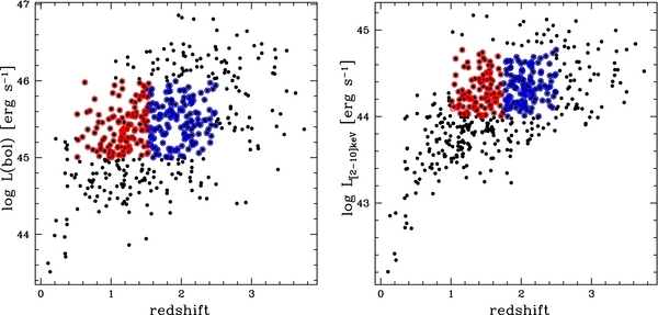
Figure 16. Left panel: distribution of Lbol as a function of redshift. Red and blue open circles mark the two subsamples at logLbol = 45–46 [erg s−1] with redshift 0.5 ⩽ z ⩽ 1.55 (136 objects) and 1.55 < z ⩽ 2.5 (139 objects), respectively. Right panel: distribution of L[2–10] keV as a function of redshift. Red and blue open squares mark the two subsamples at logL[2–10] keV = 44–44.8 [erg s−1] with redshift 1.0 ⩽ z ⩽ 1.75 (120 objects) and 1.75 < z ⩽ 2.5 (112 objects), respectively.
Download figure:
Standard image High-resolution image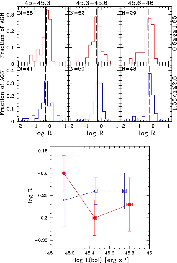
Figure 17. Upper panel: distributions of logR in bins of Lbol and redshift. The panels are divided between 0.5 ⩽ z ⩽ 1.55 (top three panels) and 1.55 < z ⩽ 2.5 (bottom three panels), and bolometric luminosities increase from left to right (logLbol [erg s−1] intervals and the number of objects are reported on top of each panel). Histograms show the observed logR distributions. The dashed lines are the median values, while the solid black lines in the first and second bins are plotted at the logR value corresponding to the median in the highest luminosity bin. Lower panel: median logR as a function of the median Lbol. Filled circles and open squares represent the median logR for 0.5 ⩽ z ⩽ 1.55 and 1.55 < z ⩽ 2.5, respectively. Solid lines connect low-redshift bins, while dashed ones connect high-redshift bins. Error bars on the median are estimated considering the MAD divided by the square root of the number of observed AGNs.
Download figure:
Standard image High-resolution image6.6.2. Evolution of the R–L[2–10] keV Relationship with Redshift
The same analysis as in the previous section has been applied to the R–L[2–10] keV relationship by binning in z and L[2–10] keV. The redshift bins are 1.0 ⩽ z ⩽ 1.75 and 1.75 < z ⩽ 2.5 in the L[2–10] keV range of 1044–44.8 erg s−1, while the luminosity cuts in each redshift bin are logLbol[erg s−1] =44–44.22, 44.22–44.5, and 44.5–44.8. In Figure 16 (right panel) the L[2–10] keV distribution as a function of redshift is presented. Red and blue open circles mark the two complete subsamples selected with the criteria above. There are 113 AGNs in the low-redshift bin with a median Lbol = 1044.25 erg s−1, while there are 120 objects in the high-redshift bin with a median Lbol = 1044.34 erg s−1. There is a factor of ∼1.2 difference, and a (two-sided) Kolmogorov–Smirnov test gives a D value of 0.19 and probability of 0.014. The histograms in Figure 18 (upper panel) show the logR distributions, while the dashed lines represent the median logR in each bin. In Figure 18 (lower panel) the median logR is plotted against the median L[2–10] keV. The two redshift bins do not show significantly different trends, and the median is consistent within the errors. The narrow range of L[2–10] keV does not allow us any claim on whether a significant evolution of R as a function of L[2–10] keV is present.
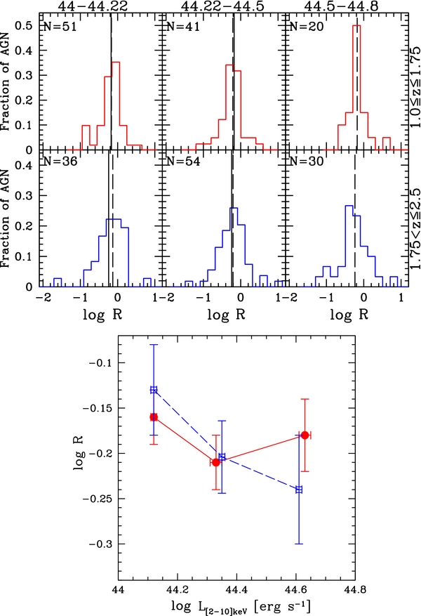
Figure 18. Upper panel: distributions of logR in bins of L[2–10] keV and redshift. The panels are divided between 1.0 ⩽ z ⩽ 1.75 (top three panels) and 1.75 < z ⩽ 2.5 (bottom three panels), and bolometric luminosities increase from left to right (logLbol [erg s−1] intervals and the number of objects are reported on top of each panel). Histograms show the observed logR distributions. The dashed lines are the median values, while the solid black lines in the first and second bins are plotted at the logR value corresponding to the median in the highest luminosity bin. Lower panel: median logR as a function of the median Lbol. Filled circles and open squares represent the median logR for 1.0 ⩽ z ⩽ 1.75 and 1.75 < z ⩽ 2.5, respectively. Solid lines connect low-redshift bins, while dashed ones connect high-redshift bins. Error bars on the median are estimated considering the MAD divided by the square root of the number of observed AGNs.
Download figure:
Standard image High-resolution image6.7. Torus Models
The presented analysis of the obscured AGN fraction over about four decades of Lbol is consistent with what has been found by demographics (i.e., S05), yet considering a completely different and independent method. This result favors the "receding torus" scenario where re-emission occurs in the optically thin torus regime. Interestingly, Hönig & Kishimoto (2011), studying the infrared emission of Type 1 AGNs through a set of simulations of clumpy torus models, have found that, although the clouds are optically thick, the visible AGN SED is dominated by optically thin dust. Increasing AGN radiation pressure may cause large thick dust clouds to be driven out of the torus at higher luminosities, and this effect can be also explained by optically thin layers of dust illuminated by the nuclear source (Hönig & Kishimoto 2010).
In the context of the receding torus, the obscured fraction can be defined as (see Simpson 1998, 2005)

where  is the luminosity for an opening angle of 60° (i.e., equal number of Type 1 and 2 AGNs), under the assumption that the height of the torus is constant with luminosity. This model for the main and low-reddening AGN sample is shown as solid lines in Figures 19 and 20 for the optically thin (left panel) and thick (right panel) torus regime. For both cases our data are not well fit by this model. Considering the main sample of 513 Type 1 AGNs (i.e., 0 ⩽ E(B − V)qso ⩽ 1), the best fit for the optically thin case has a reduced (6 degrees of freedom) χ2 of 142 for
  erg s−1, while the optically thick case has a reduced χ2 of 200 for
  erg s−1 (see Figure 19). If we instead consider the sub-sample of 391 Type 1 AGNs (i.e., E(B − V)qso ⩽ 0.1), the best fit for the optically thin case has a reduced (6 degrees of freedom) χ2 of 90 for
  erg s−1, while the optically thick case has a reduced χ2 of 177 for
  erg s−1 (see Figure 20).
We instead adopt the modified receding torus model presented in Simpson (2005), where the height of the torus is allowed to vary (h∝Lξ), and hence Equation (4) becomes

This model produces a very good fit of our data in both torus regimes. Considering the main AGN sample, the best fit for the optically thin case has a reduced (5 degrees of freedom) χ2 of 2 for  erg s−1 and ξ = 0.37 ± 0.02, while the optically thick case has a similar χ2 for
  erg s−1 and ξ = 0.44 ± 0.03 (see Figure 19). For the low-reddening AGN sample we found that the best fit for the optically thin case has a reduced (5 degrees of freedom) χ2 of 5 for
  erg s−1 and ξ = 0.32 ± 0.03, while the optically thick case has a reduced χ2 of 1.2 for
  erg s−1 and ξ = 0.43 ± 0.03 (see Figure 19). In light of this, the model employing a luminosity-dependent torus height is preferred.
As a further support to our analysis, we note that Cao (2005, C05 hereafter), considering a sample of 64 Palomar-Green (PG) QSOs with infrared SEDs (3–150 μm) observed by the Infrared Space Observatory, has estimated how the torus height varies with luminosities considering an SED-based approach.18 C05 has found that the height of the torus scales with Lbol (estimated from the optical continuum luminosity at 5100 Å and a kbol = 9) with a slope ξ of 0.37 ± 0.05. Fifty-four PG QSOs in the C05 sample have FWHM of the Hβ line larger than 2000 km s−1 (broad-line QSO sample). For this sub-sample, C05 has found a slope ξ = 0.34 ± 0.04. The fact that our best-fit ξ value agrees with that of C05 provides further (independent) evidence that a torus optically thin to its own radiation is the preferred solution.
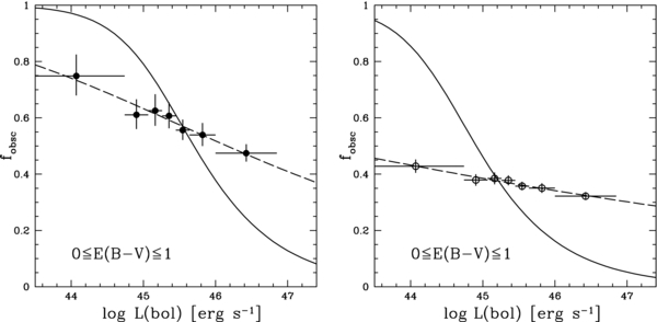
Figure 19. Obscured AGN fraction as a function of Lbol for the main AGN sample. Left panel: optically thin torus models. The solid line shows the best-fit "standard" receding torus model (Equation (4)), while the long-dashed line represents the best-fit model where the torus height varies (Equation (5)). Right panel: optically thick torus models. Line types are the same as in the left panel.
Download figure:
Standard image High-resolution image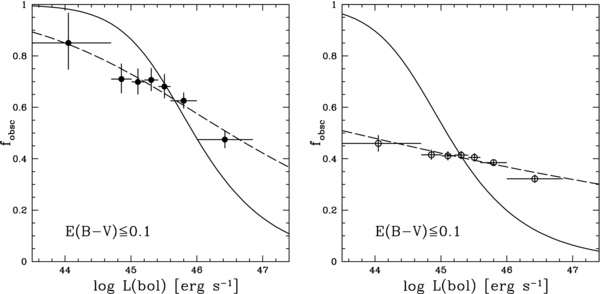
Figure 20. Obscured AGN fraction as a function of Lbol for the low-reddening AGN sample. Left panel: optically thin torus models. The solid line shows the best-fit "standard" receding torus model (Equation (4)), while the long-dashed line represents the best-fit model where the torus height varies (Equation (5)). Right panel: optically thick torus models. Line types are the same as in the left panel.
Download figure:
Standard image High-resolution imageSummarizing, our data favor the optically thin solution with the height of the torus varying with the bolometric luminosity with a slope ξ = 0.32–0.37 considering the low-reddening and the main AGN sample, respectively.
6.8. Possible Biases
Hatziminaoglou et al. (2008) pointed out that SED fitting techniques are both powerful and limited. They are powerful not only because samples with photometry are always orders of magnitude larger than the spectroscopic ones, but also because photometry allows us to explore a wider range of wavelength than a single spectrum. The limitations are, for example, in the quality of the photometric data and in the templates employed to explore the parameter space (i.e., degeneracies in the model parameters).
In our analysis we are employing only one BBB template that does not vary on the x-axes (i.e., we have assumed a fixed disk temperature). This might bias our optical–UV luminosity estimates if the shape of the BBB changed with luminosity and/or redshift, and if there is a range of disk temperatures. However, all work in the literature on AGN SEDs has found that the shape of the average AGN SED does not change with redshift and luminosity (Sanders et al. 1989; Elvis et al. 1994, 2012; Richards et al. 2006; Shang et al. 2011; Marchese et al. 2012).
For what concerns the disk temperature, our estimate of disk luminosities might be underestimated for those sources where we are not sampling the peak of the BBB, and therefore luminosity ratios might be overestimated. In order to evaluate the wavelength to which BBB peaks in the optical–UV, we have considered the relation between disk temperature, MBH, and accretion rate given by Peterson (1997, see their Equation (3.20)). Assuming an average MBH of 3 × 10⁸ M☉, an accretion rate onto the SMBH (normalized to the Eddington one) of 0.1 (Lusso et al. 2012), and a scale radius of 3 Schwarzschild radii (i.e., the innermost stable orbit), the emission of the inner part of the disk is maximum at the frequency of ∼7 × 10¹⁵ Hz, which corresponds to a wavelength of ∼430 Å. The energy peak of the BBB lies in the unobserved extreme-ultraviolet (e.g., 100–912 Å) region (e.g., see Mathews & Ferland 1987); therefore, to determine the shape and the peak of the BBB is of particular importance.
7. SUMMARY AND CONCLUSIONS
We have presented a homogeneous and comprehensive analysis of the obscured fraction for a sample of 513 Type 1 AGNs from the XMM-COSMOS survey, which has the best available multi-wavelength coverage provided in the literature, over a wide range of redshifts (0.10 ⩽ z ⩽ 3.75) and bolometric luminosities (43.47 ⩽ logLbol [erg s−1] ⩽ 46.84). The main goals of the present study are (1) to measure the AGN infrared luminosity from the torus and the optical–UV luminosity from the accretion disk, and (2) to use these measurements to determine the fraction of obscured AGNs and its dependence on luminosity and redshift. To achieve these goals, we have employed an upgraded version of the SED fitting code already presented in Lusso et al. (2011, 2012), which models simultaneously four components of the AGN SED, i.e., cold dust from the star-forming region, hot dust from the torus, optical–UV emission from the evolving stellar population, and optical–UV from the accretion disk.
The AGN obscured fraction has been obtained without assuming any bolometric correction, and we have determined its dependence on Lbol and L[2–10] keV independently. Our SED fitting approach allows us to both correct for both the effect of intrinsic AGN reddening and subtract off the contamination of the host galaxy to isolate the AGN emission. Moreover, we have explored two distinct regimes bracketing the range of physical properties of the torus, one where the dust is optically thin (fobsc = R) and the other where it is optically thick (fobsc = R/(1 + R)) to its own infrared radiation. The true AGN obscured fraction lies between these two cases (under the assumption of a toroidal obscuring region).
Given that highly extincted Type 1 AGNs (E(B − V)qso > 0.1) will have smaller Ltorus values (resulting in lower values for R), the obscured fraction that we obtain for such objects would be systematically smaller than it is in reality. We have therefore analyzed the obscured fraction for the main sample of 513 Type 1 AGNs and for the sub-sample of 391 objects with E(B − V)qso ⩽ 0.1.
The most important results obtained in the present study can be summarized as follows.
- 1.We confirm previous studies that found a decrease of the obscured fraction of Type 1 AGNs with increasing bolometric luminosity. In particular, for the main AGN sample, fobsc ranges in the optically thin case from about 0.45 to 0.75, while in the optically thick case the trend between fobsc and Lbol is much flatter, ranging from 0.30 to 0.45. For the low-reddening sample, fobsc ranges in the optically thin case from about 0.45 to 0.85, while in the optically thick case the trend between fobsc and Lbol is much flatter, ranging from 0.35 to 0.45. This decrease with Lbol can be interpreted in the context of the receding torus model, where the covering factor of the dust is reduced at high Lbol.
- 2.We favor a scenario where the torus is optically thin, with the torus height varying with bolometric luminosity (
 ). This result is supported by the agreement between the fobsc–Lbol relation estimated with our SED-based approach and S05, which has used a different sample (i.e., optically selected AGNs) and a completely independent method (i.e., demographics).
 - 3.The obscured fraction does not vary monotonically with X-ray luminosity. The fobsc–L[2–10] keV relationship in the optically thick case is almost flat. X-ray demography-based studies found an obscured fraction lower by a factor ∼2 in the optically thin regime and by a factor of ∼1.3 in the thick one. We argue that X-ray studies miss a large fraction of the highly obscured Compton-thick AGNs at L[2–10] keV > 1044 erg s−1.
- 4.We do not find any clear evidence of evolution with redshift of the mid-infrared to bolometric luminosity ratio, and hence of the obscured fraction, as a function of both Lbol and L[2–10] keV.
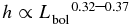
We conclude that the major driver of the fobsc −luminosity relationship is the bolometric luminosity, rather than X-ray luminosity. This is expected in the receding torus scenario, i.e., the X-ray emission is not providing most of the heat that sublimates dust and regulates the torus distance.
Our fobsc measurements could be used in the context of future demographic analyses in order to check whether AGN surveys are missing highly obscured Compton-thick AGNs. Moreover, by comparing any unbiased demographic sample to our results one could obtain deeper insights into the structure of the torus. Indeed, our comparison with S05 suggests that the torus is optically thin to its own radiation.
This analysis also provides a fitting formula (Equation (5); see Section 6.7), which can be used in all future bolometric luminosity function papers (e.g., Hopkins et al. 2007), to determine the contribution of the obscured accretion as a function of bolometric luminosity and to study the growth history of SMBHs.
We thank the anonymous reviewer for thoroughly reading the paper and providing valuable comments. We acknowledge financial contribution from the agreement ASI-INAF I/009/10/0 and from the INAF-PRIN-2011. This research is based on observations made with ESO telescopes at the La Silla or Paranal Observatories under program ID 175.A-0839. E.L. is indebted to Micol Bolzonella for providing very helpful and constructive comments on the code presented here. E.L. gratefully thanks Marco Mignoli for providing the zCOSMOS spectra for the XMM-COSMOS sources. E.L. also gratefully thanks Andrea Merloni, J rg-Uwe Pott, Elisabete de Cuhna, Brent Groves, and Angela Bongiorno for useful discussions. We also thank the members of the ENIGMA group19 at the Max Planck Institute for Astronomy (MPIA) for helpful discussions. J.F.H. acknowledges generous support from the Alexander von Humboldt Foundation in the context of the Sofja Kovalevskaja Award. G.T.R. acknowledges the generous support of a research fellowship from the Alexander von Humboldt Foundation at the Max-Planck-Institut f
 r Astronomie and is grateful for the hospitality of the Astronomisches Rechen-Institut. Support for the work of E.T. was provided by the Center of Excellence in Astrophysics and Associated Technologies (PFB 06), by the FONDECYT regular grant 1120061, and by the Anillo project ACT1101.
APPENDIX A
We summarize below the main properties of the SEDs of the outliers marked with orange open squares in Figures 5, 6, and 7.
APPENDIX B: EXAMPLES OF OUTLIERS IN THE SED FITTING SHOWN IN Figure 5
Representative examples of SEDs of outliers plotted in the left panel of Figure 5 are shown in Figure 21. The majority of them are fitted with a reddened BBB, while the optical–UV emission is mainly coming from a young stellar population. From Figure 1 it is clear that a (partial) modeling degeneracy between reddened disks and star-forming galaxies is present in the optical–UV. To break this degeneracy, an independent measurement of the host galaxy emission is needed, but it is not straightforward to estimate for unobscured AGNs. We have then tried to verify whether the best-fit SED and the optical spectrum are qualitatively in agreement. The optical spectra of these outliers are therefore fitted considering a set of SDSS composite spectra from Richards et al. (2003), representative of the quasar emission, and a grid of 39 theoretical galaxy template spectra from Bruzual & Charlot (2003, hereafter BC03), spanning a wide range in age and metallicity, to account for the stellar component. Five spectra, mainly at low Lbol, obs, have poor signal-to-noise ratio, and therefore it is not possible to obtain a reasonably good fit for them. Four sources can be fitted only if, along with an SDSS reddened quasar composite, a significant host galaxy component is also included. For three objects (see the SED of XID = 54513, 2072, and 5323) there is no detectable host galaxy component, and the spectrum is well fitted with an SDSS quasar composite spectrum alone, although one of the reddest composite spectra. The SEDs are presented in Figure 21, and some spectra examples from zCOSMOS 20k-Bright (Lilly et al. 2007; S. J. Lilly et al., in preparation) are presented in Figure 22, where we show the SDSS reddened quasar composite spectrum for clarity. The best-fit SEDs of these objects are not in agreement with the spectral fit.
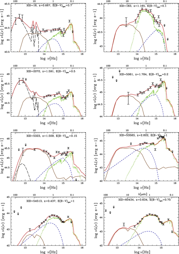
Figure 21. Examples of outliers in the SED fitting shown in Figure 5. Lines and symbols are the same as in Figure 3.
Download figure:
Standard image High-resolution image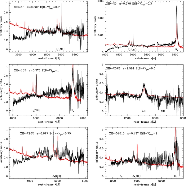
Figure 22. Examples of spectra of heavily reddened Type 1 AGNs (zCOSMOS 20k-Bright; Lilly et al. 2007; S. J. Lilly et al., in preparation) in the analyzed sample with identification of the main emission lines. The flux is per unit wavelength (Fλ), and normalization is arbitrary. The red line is the SDSS reddened quasar composite (Richards et al. 2003).
Download figure:
Standard image High-resolution imageAs a further sanity check, we have fitted the whole sample without the host galaxy component. The scatter in the logLbol, obs/Lbol distribution is obviously smaller with a median logLbol, obs/Lbol of 0.20. The average obscuring fraction and the results discussed in our analysis are not significantly affected.
APPENDIX C: EXAMPLES OF OUTLIERS IN THE SED FITTING SHOWN IN Figure 6
The upper outliers in Figure 6 are shown in the top-middle row of Figure 23. On average, these objects present very high reddening (E(B − V)qso ⩾ 0.7) and NH values of the order of ∼1022 cm−2. The optical spectrum of XID = 135 (NH ≃ 1.1 × 1022 cm−2) shows a strong [O iii] emission line, a faint/absent Hβ, but the Hα is broad. The high Hα/Hβ ratio (≫3) indicates high reddening, consistent with the best-fit BBB SED (see Figure 22, middle left). The spectrum of XID = 447 (NH ≃ 7 × 1022 cm−2) has a poor signal-to-noise ratio, but it shows a broad Mg ii. XID = 2152 (NH ≃ 1.2 × 1021 cm−2) has a strong narrow Hβ emission line on top of a broad component with an FWHM ∼ 2000 km s−1 (see Figure 22, bottom left). The continuum of this source shows a high level of obscuration, consistently with the results from our SED fit. The spectrum of XID = 5205 (NH ≃ 1.2 × 1023 cm−2) has a good signal-to-noise ratio and shows broad emission lines, however with some level of reddening, in agreement with our SED fit. These four AGN might be considered intermediate-type AGNs (1.5 to 1.9). For the other five outliers, three have a photometric redshift, while for the two with spectra similar considerations can be made: either the spectrum has a poor-signal-to-noise ratio but with broad lines present, and/or lines show intermediate FWHM (∼2000 km s−1).
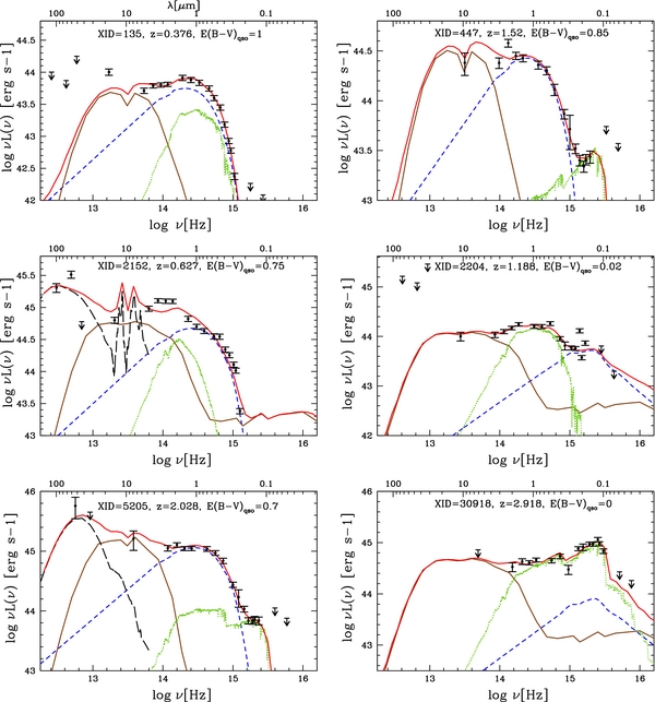
Figure 23. Examples of outliers in the SED fitting shown in Figure 6. Line types are the same as in Figure 3. Top-middle row: outliers at more than 3σ above the median. Bottom row: outliers at more than 3σ below the median.
Download figure:
Standard image High-resolution imageThe SEDs of the lower outliers in Figure 6 are presented in the bottom row of Figure 23. The spectrum of XID = 30918 has a good signal-to-noise ratio with evident broad-line features (e.g., broad C iv). XID = 2204 is clearly a broad-line AGN (broad Mg ii), in agreement with the best fit, although a significant host galaxy contamination is present.
APPENDIX D: EXAMPLES OF OUTLIERS IN THE SED FITTING SHOWN IN Figure 7
The upper outliers in Figure 7 are presented in the top row of Figure 24. These objects present an SED with a strong near-infrared bump. The SED of XID = 5607 was already discussed in Hao et al. (2013) and was presented as a good candidate for an AGN at the beginning of the "blow-out phase," where the nucleus emerges from its dusty cocoon and starts dominating in the optical–UV. However, we caution the reader that the Ltorus values for these two outliers are uncertain given that these sources do not have a 24 μm detection.
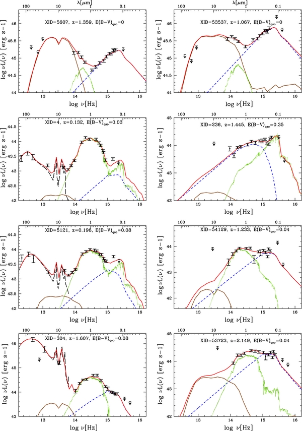
Figure 24. Examples of outliers in the SED fitting shown in Figure 7. Line types are the same as in Figure 3. Top row: outlier at 3σ above the median of the 〈logLIR, obs/Ltorus〉 distribution (right panel of Figure 7). Second and third rows: outliers at 3-σ below the median at LIR, obs < 1044.6 erg s−1. Bottom row: outliers at 3-σ below the median at LIR, obs > 1044.6 erg s−1.
Download figure:
Standard image High-resolution imageExamples of outlier SEDs at LIR, obs < 1044.6 erg s−1 are presented in the second and third rows of Figure 24. These sources are strongly galaxy dominated with weak near-infrared emission coming from the torus, and all of them have MIPS detection at 24 μm. At LIR, obs > 1044.6 erg s−1 outliers still show a strong galaxy emission, but the disk is clearly present (see bottom row in Figure 24). Eight sources in this region do not have 24 μm detection, making these estimates uncertain (as shown by the large error bars), while six sources also have Herschel data and an SED similar to XID = 304 (z = 1.607) plotted in Figure 24. The latter object has a best-fit torus luminosity of Ltorus = 1044 erg s−1, much lower than what is measured from the observed SED (LIR, obs = 1045.6 erg s−1). In our fit this source appears to be a composite AGN/starburst SED, where the AGN component is extremely weak in comparison with the starburst one. This is in good agreement with the results presented by Hao et al. (2013). In this paper XID = 304 has been fitted by a ULIRG Arp 220 SED (Polletta et al. 2007), but weak broad emission lines are present in the spectrum. This result has been interpreted by Hao and collaborators as evidence for a "new born quasar," where the AGN starts becoming visible during a merger triggered starburst (Hopkins et al. 2006). We cannot exclude this possibility, but a detailed separate analysis is required (H. Hao et al., in preparation).
Footnotes
- 9
In the following we will not make any distinction between emission from the torus and the emission from the hot dust.
- 10
The multi-wavelength XMM-COSMOS catalog can be retrieved from http://www.mpe.mpg.de/XMMCosmos/xmm53_release/, version 2011 November 1. This is an updated version of the catalog already published by Brusa et al. (2010), which includes the photometric redshift catalog by Salvato et al. (2011) and new spectroscopic redshift measurements.
- 11
A definition of the dust-reddened Type 1 AGN sample in XMM-COSMOS was already presented in Lusso et al. (2010). Their Figure 13 clearly shows that ∼10%–20% of the AGN population in XMM-COSMOS has E(B − V)qso > 0.1. This dust-reddened AGN population also presents colors that are redder than what has been found by Richards et al. (2003, see their Figure 6).
- 12
We are implicitly assuming that the observed soft and hard X-ray emission originated on scales smaller than that of the torus.
- 13
Column densities lower than 1022 cm−2 are almost transparent to hard (>2 keV) X-rays (Morrison & McCammon 1983).
- 14
The SED for XID = 300 (COSMOS
J100050.16+022618.5, z = 3.715) is fitted with a starburst galaxy, but presents clear QSO features in the spectrum (Lyα, C iv). The observed SED has very strong BBB with absorption at wavelength shortward of 912 Å, but the SED fitting code is not able to reproduce this feature with a reddened disk. The SED for XID = 2394 (COSMOSJ100127.53+020837.8, z = 3.333) is very well fitted with a star-forming galaxy, and the spectrum presents a faint AGN feature (C iv). - 15
The MAD term is the median of the absolute deviation between the data and the median of the data (MAD = 〈ABS(d − 〈d〉)〉, where d's are the data). The MAD value is scaled by a factor of 1.483 to become comparable with the Gaussian standard deviation.
- 16
In this case, the Lbol values (output of our code) have the AGN reddening left in. The LIR, obs and Ltorus values are consistent within 0.16 dex, but the reddened Lbol estimates are, on average, lower than Lbol, obs.
- 17
S05 classified objects that display broad (FWHM > 1000 km s−1) Hα and Hβ emission lines as Type 1 AGNs, while objects showing only broad "wings" of the Hα line were classified as intermediate Type 1 and grouped into the Type 2 AGN sample.
- 18
That is, through the fobsc–Lbol relation with fobsc = LIR, obs/Lbol. The host galaxy/reddening contribution is neglected given that these objects are bright PG QSOs with Lbol ∼ 1045–47 erg s−1. The C05 sample contains also two QSOs with Lbol ∼ 1048 erg s−1.
- 19

