


ABSTRACT
A Fourier transform analysis of 2.5 million spectra in the SDSS survey was carried out to detect periodic modulations contained in the intensity versus frequency spectrum. A statistically significant signal was found for 223 galaxies, while the spectra of 0.9 million galaxies were observed. A plot of the periods as a function of redshift clearly shows that the effect is real without any doubt, because the modulations are quantized at two base periods that increase with redshift in two very tight parallel linear relations. We suggest that this result could be caused by light bursts separated by times on the order of 10−13 s, but other causes may be possible. We investigate the hypothesis that the modulation is generated by the Fourier transform of spectral lines, but conclude that this hypothesis is not valid. Although the light burst suggestion implies absurdly high temperatures, it is supported by the fact that the Crab pulsar also has extremely short unresolved pulses (<0.5 ns) that imply similarly high temperatures. Furthermore, the radio spectrum of the Crab pulsar also has spectral bands similar to those that have been detected. Finally, decreasing the signal-to-noise threshold of detection gives results consistent with beamed signals having a small beam divergence, as expected from non-thermal sources that send a jet, like those seen in pulsars. Considering that galaxy centers contain massive black holes, exotic black hole physics may be responsible for the spectral modulation. However, at this stage, this idea is only a hypothesis to be confirmed with further work.
Export citation and abstract BibTeX RIS
1. INTRODUCTION
The time domain is the least explored of all the physical astronomical domains (Fabian 2010). This fact is particularly the case for short timescales. The 2 ns pulses and the unresolved (<0.5 ns) nanopulses observed in the Crab pulsar (Hankins et al. 2003; Hankins & Eilek 2007) are the shortest astrophysical time signals observed. Lorimer et al. (2007) reported a single 5 ms powerful burst of radio emission and searches for fast radio transients are presently being carried out with Very Long Baseline Array data (Wayth et al. 2011). Astronomical objects that vary within times shorter than nanoseconds could be detected by searching for periodic modulations in their spectra (Borra 2010). Borra (2010) showed that objects that emit brief intensity pulses separated by times shorter than 10−10 s induce spectral modulations detectable in astronomical spectra. The basic concept of the theoretical analysis in Borra (2010) can be intuitively understood by considering that the spectrum of a light source is given by the Fourier transform of the fluctuations of the electric field as a function of time (Klein & Furtak 1986). If we have two pulses of light separated by a time t, the spectrum will be modulated by a cosine because the Fourier transform of two separate peaks gives a cosine. Note, however, that a spectral modulation does not have to be generated from only two pulses. Rather, a modulation can be generated by a large number of pairs of pulses separated by the same constant time t, but with each pair emitted with time separations much larger than t that could be periodic with a period much larger than t, or even emitted at random times much larger than t (Borra 2010). This fact is an important remark because a signal generated from only two pulses would imply an extremely large energy emitted in a very short time. The experiments of Chin et al. (1992) support the theoretical analysis in Borra (2010). The present paper discusses some of the results of a Fourier transform analysis of 2.5 million astronomical spectra in the Sloan Digital Sky Survey carried out to detect spectral modulations (Trottier 2012). Although the original motivation for the survey was to look for spectral modulations caused by ultrarapid light bursts, spectral modulations could also be caused by other effects. For example, we consider, in the present paper, two possibilities: instrumental effects and the effect of the Fourier transform of spectral lines. We conclude that these two effects do not apply. We do not know of any other possible causes of spectral modulations.
2. DATA ANALYSIS
To search for the type of signal caused by intensity pulses with short time separations (Borra 2010), a Fourier transform analysis of 2.5 million spectra in the Sloan Digital Sky Survey (SDSS) was carried out to detect periodic modulations contained in their frequency spectra (Trottier 2012). The Fourier transform is conducted in the frequency domain, which gives a Fourier spectrum in the time domain. This procedure can be confusing since the language commonly used in textbooks is for Fourier transforms applied in the time domain, producing a Fourier spectrum in the frequency domain. Therefore, we emphasize that, in this paper, we will use the word "frequency" to refer to the units in the frequency spectrum before the Fourier transform. The units become time units after the Fourier transform of a frequency spectrum; however, in the discussion and the figures, we shall use the sampling number N, instead of time, so that the sampling can clearly be seen. Using time units would have been confusing in the discussion. The sampling number N can be converted to time units (seconds) by multiplying by 2.1 × 10⁻¹⁵. The period in Hertz units in the frequency spectrum is therefore given by 1/(2.1 × 10−15 N).
The SDSS spectra were first converted to frequency units because the expected spectral modulation is periodic in frequency units (Borra 2010). This procedure was done with the usual relations ν = c/λ and Δν = cΔλ/λ2. Furthermore, a Fourier transform carried out in the frequency domain requires that the spectrum be equally sampled in frequency. However, the SDSS spectra are equally sampled in wavelength, so they are not equally sampled in the frequency domain. Consequently, a linear interpolation using the observed values on both sides of the required values, after conversion from wavelengths to frequencies, was used to generate equally sampled values in frequency. The spectra were then analyzed using Fast Fourier Transform (FFT). Because the number of spectra is very large, simple signal finding algorithms must be used. A frequency spectrum is first smoothed with the Matlab function "smooth" which uses a moving average filter. The smoothing length used is equal to 2.5% of the total length of the spectrum. This 2.5% length was chosen, after numerical experimenting, to ensure that it removes the short periods in the frequency spectra (corresponding to high values of N in the Fourier domain), but does not remove the long periods (corresponding to low values of N). The smoothed spectrum is then subtracted from the unsmoothed one and the FFT performed on the difference between the unsmoothed and the smoothed spectra. This technique was used after experimenting with Fourier transforms of spectra without subtractions of the smoothed continuum and with subtractions of the smoothed continuum, including actual spectra and numerical simulations. The reason why the smoothed spectrum is subtracted is that, otherwise, there is a very strong and bumpy contribution at low values of N (N < 40) that would make it extremely difficult to detect a signal with software that analyzes an extremely large number of spectra (millions) and consequently must use simple numerical algorithms. In principle, one could simply cut off the region at low N; however, after trial and error, it was found that subtracting the smoothed spectrum (and therefore low values of N in the Fourier domain) gave better results. For example, smoothing in the frequency domain does not abruptly remove values of N below a cutoff value but in stead removes them gradually as a function of N below a desired N removal value. This procedure allows one to see the Fourier spectrum even at low values of N and to use simple numerical algorithms. This smooth transition with N, that occurs at N < 40, can be seen in Figures 1, 2, 5, and 7 that show Fourier transforms of the spectra. A frequency spectrum where the smoothed spectrum has been subtracted is also easier to inspect visually (see Figures 6 and 8). Comparisons of Fourier transforms of spectra with and without subtraction of the smoothed frequency spectrum, including numerical simulations, show that the subtraction does not remove signals for periods above the desired removal value and does not introduce artificial signals. An SDSS spectrum typically contains 3900 digital samplings in the frequency domain and therefore yields, after the FFT, 1950 samplings in the time domain. The FFT is carried out with the FFT function "fft" in Matlab software. The algorithms used by the function "fft" are explained in detail in the help section of Matlab. In this paper, we only consider the Fourier modulus that best characterizes the power of a signal and is always positive. Figure 1 shows the Fourier transform of the spectrum of a bright galaxy at R.A. = 50.53610 and decl. = −0.83626 (J2000) that has a strong signal. The signal at N = 54 (corresponding to a time t = 1.13 × 10⁻¹³ s) is very sharp (only one sample), as expected after the Fourier transform of a periodic modulation that covers the entire spectral range observed. The Fourier modulus is plotted as a function of the sampling number N, instead of time, so that the sampling can clearly be seen. Beyond N = 500, the N dependence of the Fourier modulus is essentially flat, within the noise, because it is dominated by white noise and shows the type and amplitude of fluctuations one sees for 400 < N < 500 in Figure 1. This result is the case for the majority of the SDSS objects and it is always the case for galaxies. In time units, N = 1 corresponds to 2.1 × 10⁻¹⁵ s and time increases linearly with N. Note that the total energy contained in the signal is actually not as strong as it appears because most of the energy is contained in the subtracted smoothed spectrum. Also, the 3 arcsec diameter of an SDSS fiber only samples a small fraction (the core) of this extended (about 1 arcmin) low-redshift (z = 0.0365) galaxy. To better display the shape of the signal, Figure 2 plots the first 100 samples of the Fourier transform in Figure 1. This figure clearly shows that the signal at N = 54 is one sample wide. As discussed later, this characteristic is a very important property of all the signals detected.
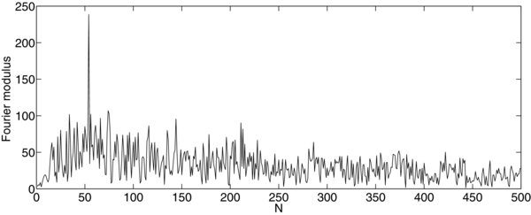
Figure 1. Fourier transform of the frequency spectrum (after subtraction of its smoothed frequency spectrum) of the core of a bright galaxy with a strong signal. The FFT modulus is plotted as a function of the FFT sampling number N. Only the first 500 samples (out of 1950) are plotted so that the signal at N = 54 (1.13 × 10⁻¹³ s in time units) can clearly be seen. In time units N = 1 corresponds to 2.1 × 10⁻¹⁵ s and time increases linearly with N. The subtraction of the smoothed spectrum removes the strong contribution present in the FFT of the unsmoothed spectrum for N < 20 (see Section 2).
Download figure:
Standard image High-resolution image
Figure 2. First 100 samples of the Fourier transform spectrum in Figure 1. The signal at N = 54 (1.13 × 10⁻¹³ s) is very sharp (only one sample), as from the Fourier transform of a periodic spectral modulation that extends at least over the entire SDSS spectrum.
Download figure:
Standard image High-resolution imageTo detect the type of signal seen in Figures 1 and 2, the software flags objects that have a peak, in the FFT spectrum, with a signal-to-noise ratio greater than a preset value. The signal is the signal of a single Fourier sample, the noise is evaluated with Equation (2), and the signal-to-noise ratio is the ratio between these two numbers. Only a single sample is used by the software because its purpose is only to extract the Fourier transform spectra that have a statistically significant signal. Each extracted Fourier spectrum can then be visually inspected so that the presence of other significant samples can also be considered. The software is written in a homemade Matlab code to analyze SDSS spectra, but it also uses Matlab functions: for example, the functions "smooth" to carry out the smoothing and "fft" to carry out the FFT. The software was extensively tested on SDSS spectra as well as numerical simulations. Because the modulus of the FFT is used, a statistical analysis must use Rayleigh statistics, which have the cumulative distribution function

where σ is the standard deviation. To evaluate the noise, a Fourier spectrum is divided into eight separate contiguous boxes of 250 Ii samples and the standard deviation σ is computed for every box from the relation that must be used for Rayleigh statistics:
This value of σ is then used for all locations within that box. The box at the highest values of N has fewer than 250 samples (usually about 200) since eight boxes of 250 samples cannot fit within the typical 1950 samples in the Fourier spectrum. No attempts are made to subtract the underlying "continuum" contribution coming from the Fourier transform of the frequency spectrum from the values of Ii used to compute the standard deviation in Equation (2) and to compute the signal. We adopt this procedure because, first, the underlying Fourier "continuum" is small for N > 250, even for bright objects, and contributes little to Ii and therefore the signal-to-noise ratio. For N > 500, the background signal is dominated by white noise for the majority of spectra and for all galaxies. For example, the Fourier spectrum in Figure 1 continues to show, for N > 500, a noisy appearance similar to what is seen for 400 < N < 500. Second, for N < 250, the continuum, which is negligible for faint objects (mostly galaxies) but significant for bright ones (mostly stars), must be evaluated from a bumpy Fourier modulus (as in Figures 1 and 2 but without the signal at N = 54) and depends on the spectral type of the object. It would therefore be extremely difficult to evaluate the contribution of the continuum with software that runs without human intervention, as needed because of the huge quantity of spectra analyzed (2.5 million). In the evaluation of σ for N < 250 and for bright objects, the underlying bumpy continuum signal therefore contributes to the noise evaluated from Equation (2) and thereby decreases the signal-to-noise ratio. On the other hand, failing to remove the continuum has the opposite effect of adding a contribution, thereby increasing the signal. In practice, to avoid having to visually inspect too large a number of detections, only peaks with a signal-to-noise ratio >6.5 were used for N < 250 because there would otherwise have been too many detections of trivial signals that would have to be visually inspected. These detections would have come from spectral bumps in very bright objects, mostly bright early-type stars (see Figure 5 for an example). Although the detection method has flaws for bright objects (mostly bright stars) and N < 250, these flaws are not important at this stage of the search, where the main purpose is to find whether peculiar objects exist; we are less concerned with a quantitative estimate of their occurrence rates. The software therefore simply flags interesting objects that can then be individually inspected. Note that these flaws are mostly important for stars, which tend to have bright spectra in the SDSS database. These flaws are not important for galaxies because most galaxies are faint and, furthermore, the 3 arcsec diameter of an SDSS fiber only samples a fraction of their apparent diameters. Consequently, there is a small continuum contribution in the FFT spectra from the brightest galaxies, even for N < 250 (see Figure 1).
3. RESULTS
The analysis for N > 250 produced several detections, consistent with Rayleigh statistics. For N < 250, a remarkable pattern, shown in Figure 3, is apparent for the signals detected in galaxies. The spectra of 0.9 million galaxies were analyzed (many galaxies were observed on different Julian dates) but signals were detected in only 223 of them for a signal-to-noise ratio >6.5. Figure 3 shows that the positions of the detected signals increase linearly with redshift along two linear staircases that have their bases (for a redshift z = 0.0) at N = 52 (time = 1.09 × 10⁻¹³ s) and N = 49 (time = 1.03 × 10⁻¹³ s). The staircases are consistent with a tight linear relationship sampled at the integer values of N given by the FFT. The staircase is caused by the effect of the discrete sampling in N. A linear relationship as a function of redshift signifies that the period of the spectral modulation is universal in the reference frame of the galaxies. On the one hand, this result clearly shows that the signal is real and not an instrumental or data reduction artifact; on the other hand, this result places severe constraints on its cause. The upper staircase relationship (with a base at N = 52) shows that the signals are very sharp, similar to the signal seen in Figure 2. If the signals were broad (with width ΔN > 1), the steps would not be so well defined. The staircase is therefore consistent with a spectral modulation, present in the entire observed spectrum of the galaxies, that has the same value of N in their reference frame and increases linearly with redshift as observed on Earth. This effect can also be seen in the lower staircase, although it is not as well defined because of the smaller number of galaxies.

Figure 3. Signals detected in galaxies as a function of redshift. The positions of the signals increase linearly with redshift along two linear staircases that have their bases (for a redshift z = 0.0) at N = 52 (1.09 × 10⁻¹³ s) and N = 49 (1.03 × 10⁻¹³ s).
Download figure:
Standard image High-resolution imageAs discussed in Section 2, the evaluation of the signal and the noise for N < 250 includes the contributions of the continuum. It was previously stated that this effect does not have a significant impact on the results. The statistical analysis that follows quantitatively elaborates on this assertion. First, assuming that the periodic signal in Figures 1 and 2 is superposed on a background value equal to the continuum of the underlying Fourier spectrum, we find that the net signal has an amplitude of I = 130. Because the Fourier transform of white noise (photon noise in our case) also gives white noise, we can evaluate the standard deviation at large values of N, where the contribution from the Fourier continuum is totally negligible, and then apply it to an evaluation of the signal-to-noise ratio at N = 54. The white noise standard deviation is 8.0 for that spectrum, giving a signal-to-noise ratio of 16.25 for the signal and, using Equation (1), a probability of 6.1 × 10⁻³⁴ of detecting a signal generated by random noise. Considering that 2.5 × 10⁶ SDSS spectra were analyzed, this result gives a probability = 1.5 × 10⁻²⁷ that a signal generated by random noise is in a spectrum of an object at a given N location. There are a few other objects that give comparable results. Second, three of the galaxies in Figure 3 were detected with a signal-to-noise ratio >7.30. A visual examination of their Fourier spectra shows that the contribution I of the underlying Fourier continuum of these faint galaxies is negligible so that the computed signal-to-noise ratio is reasonably accurate. Equation (1) gives a probability = 2.3 × 10⁻¹² that the signal is due to random noise. Considering that 2.5 × 10⁶ SDSS spectra were analyzed, this result gives a probability = 5.8 × 10⁻⁶ that a signal generated by random noise is in a spectrum of an object at a given N. The probability that three signals are detected from random noise is given by the product of the three probabilities and is therefore totally negligible.
To see the effect of lowering the signal-to-noise ratio selection minimum, a subsample of 128,000 spectra (5% of the total number) were analyzed again, but with the signal threshold detection lowered to a signal-to-noise ratio >6.0. The subsample is composed of spectra all in the same region of the sky, so no selection effect is present. Signals were detected in 83 galaxies, 19 of which have a signal-to-noise ratio >6.5. The positions of the detected signals as a function of redshift are plotted in Figure 4. These data show the same staircase relationships seen in Figure 3. Because the spectral subsample contains 5% of the total number of spectra analyzed, we can estimate that lowering the signal-to-noise threshold to 6.0 for the entire survey would have yielded 1660 detections instead of 223, thus increasing the number of detections by a factor of 7.4. The fact that decreasing the signal-to-noise ratio of the detection threshold to 6.0 from 6.5 would only increase the number of detections by a factor of 7.4 while Rayleigh statistics (Equation (1)) predict a factor of 23 is consistent with a very small fraction of galaxies having strong signals. The remainder of galaxies must have a substantially smaller signal or perhaps no signal all. Note that the majority of the detected galaxies, unlike the galaxy in Figures 1 and 2, are faint, so that the continuum contributions to the signal-to-noise ratios are small.
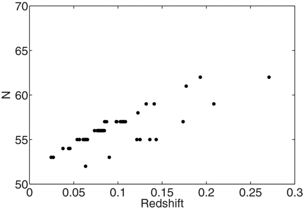
Figure 4. Positions of the signals detected in galaxies as a function of redshift for a subsample of 128,000 spectra that was analyzed again but with the threshold of signal detection lowered to a signal-to-noise ratio >6.0.
Download figure:
Standard image High-resolution imageIn conclusion, there is no doubt that a statistically significant signal has been found in a small number of galaxies. Only galaxies showed this signal, while none of the stars and none of the quasars had statistically significant signals. Furthermore, the signal was found in a very small fraction of the galaxies observed.
4. CONSIDERATION OF INSTRUMENTAL EFFECTS AND SIGNALS FROM THE FOURIER TRANSFORM OF SPECTRAL LINES
One must consider the possibility that the signals could be caused by instrumental effects. For example, the interference between two beams generated by reflections at two glass interfaces could generate the type of spectral modulations detected. However, because only a small number of galaxies were detected, while no stars nor quasars were, and the redshift relations in Figures 3 and 4 show the patterns that they do, we can exclude the possibility that the peaks are due to instrumental effects. The next two paragraphs discuss the likelihood of instrumental effects.
An instrumental effect would be likely if the detected objects were always located in the same fibers; however, this is not the case as the detected objects are located in random fibers. The detected signals are weak, in comparison to the total energy in the spectrum, and an instrumental effect should therefore be prevalently detected in bright objects, while this result is not the case. Although the SDSS contains a large number of spectra of stars considerably brighter than the detected galaxies, the signal of the spectral modulation was not detected in any of the stellar spectra. Furthermore, the detected galaxies are not particularly bright among the galaxies in the SDSS survey. As a matter of fact, many of the detected galaxies are very faint; a very large number of galaxies are brighter than the average detected galaxy. Consequently, if the signal is due to an instrumental effect, these galaxies should show the signal. However, they do not.
The tight linear redshift relations seen in Figures 3 and 4 also make an instrumental effect highly unlikely since an instrumental effect showing a periodic modulation in frequency units (e.g., interference between two optical beams) would be expected to produce a period that is constant in the reference frame of the instrument and independent of redshift. The fact that there actually are two relations, which imply two signals with different periods at a redshift z = 0.0, makes an instrumental effect even more unlikely, since one would expect both signals to be present in all detected objects, while an inspection of the Fourier spectra of all the detected objects shows that they only have a single signal. Considering that the effect of redshift is to shift to lower frequencies in the energy distribution to the reference frame of the detector, a hypothetical instrumental effect should be tied to the frequency dependence of the spectrum. However, the redshifts of the galaxies are small (half of the objects in Figures 3 and 4 have redshifts below 0.1), so that the effect of the redshift on the energy distributions is very small and unlikely to produce such tight relationships with redshift. Furthermore, there is a great diversity of spectral types among the detected galaxies. The effect should be more detectable in the bright galaxies but it is not. The fact that Figures 3 and 4 show that the redshift dependence consists of two very close parallel lines makes a redshift-dependent instrumental effect even less likely since it would imply two different quantized spectral types. A visual inspection of the galaxies in Figures 3 and 4 showed a variety of spectral types (e.g., spectra of elliptical galaxies, emission-line galaxies, etc.), similar to the spectral types of undetected galaxies.
A staircase relation like the upper one in Figure 3 could occur if a peak centered at the required location was present in the Fourier spectrum of many galaxies. The small number of detections would then be due to the effect of noise fluctuations. A by-eye inspection of the Fourier transforms of randomly chosen galaxies that were not detected and SDSS galactic templates does not support this hypothesis. The Fourier spectra typically have bumpy structures like those seen in Figures 1 and 2 (without the signal at N = 54), but do not show evidence of higher peaks at the locations predicted by Figure 3. Figure 7 shows the Fourier spectrum of an undetected galaxy. This hypothesis is also contradicted by the effect of decreasing the threshold of detection from 6.5 to 6.0, which increases the number of detections by a factor significantly smaller than that predicted by Rayleigh statistics (see Section 3).
There is a potential effect that could come from the Fourier transforms of spectral lines. The FFTs of the spectra of A and B stars that have strong absorption lines show a strong peak at N = 37 and a second weaker one at N = 57. Figure 5 shows the Fourier transform of the spectrum of an A0 star. This is a typical Fourier spectrum one obtains from the FFT of A and B stars. It shows that the peak is broad (five samplings) and that there is also a second weaker peak at N = 57. O stars also have a strong broad peak at N = 45 and a weaker peak at N = 62. Computer simulations of artificial spectra that contain absorption lines show that the peaks are due to the FFT of the contribution of the absorption lines. The simulations also show that the locations of the peaks vary linearly with redshift, leading to the suspicion that the relations in Figures 3 and 4 are due to the Fourier transform of spectral lines. However, the analyses that follow show that this is not the case. In reading the discussions in this paper, one has to consider that the spectra of the SDSS have low spectral resolution (1800–2000, which corresponds to about 2.5 Å) and low signal-to-noise ratios (Figures 6 and 8 show these facts for two bright galaxies); consequently, to be detected in an SDSS spectrum, spectral lines would have to be strong. A visual comparison of the spectra of detected galaxies with the spectra of hundreds of galaxies that were not detected did not show any noticeable difference, within the noise in the spectra, in the absorption or emission lines present in the spectra. The detected galaxies had unremarkable spectra. This result is also true of the spectrum of the galaxy that gave the strong signal seen in Figures 1 and 2. A visual inspection of the spectra of the detected objects on the SDSS website shows that they are also, within the noise, well fit by SDSS spectrum templates and that their spectral lines are identified as being common spectral lines. Some of these spectra have emission lines, but the majority do not. The strengths of the emission lines vary greatly among the few detected galaxies with emission lines. There also is a diversity of galaxy types among the detected galaxies in Figure 3 (e.g., elliptical, emission line, star forming). Furthermore, the 3 arcsec diameter of the SDSS fiber samples a large fraction of the diameters of the faint distant galaxies but only the nucleus of the nearby ones (e.g., the galaxy used to generate Figures 1 and 2). Note also that, unlike early-type stars, the FFTs of later stellar spectral types, which are more representative of the spectra of detected galaxies, do not show significant peaks. In conclusion, on the basis of the by-eye inspection of the spectra, the detected galaxies do not show striking trends that differentiate them from the undetected galaxies.
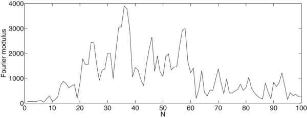
Figure 5. Fourier transform of the frequency spectrum (after subtraction of its smoothed frequency spectrum) of a bright A0 star. Only the first 100 values of N are plotted.
Download figure:
Standard image High-resolution image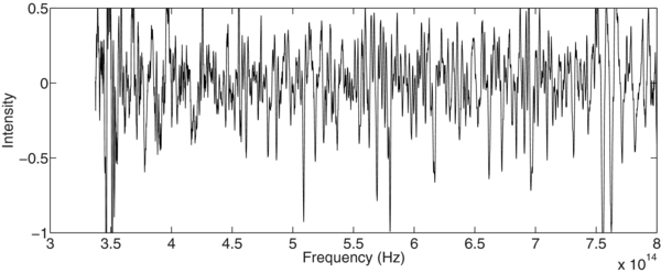
Figure 6. Spectrum of the galaxy in Figures 1 and 2, in frequency units, after subtraction of the smoothed continuum. The spectrum was blueshifted to a redshift z = 0.0 to facilitate a comparison with Figures 8 and 11. The amplitude of the detected periodic signal is ± 0.2 in the frequency spectrum, so the signal is buried in noise and one would not expect to recover the signal in a simple visual inspection.
Download figure:
Standard image High-resolution imageFigure 6 shows the frequency spectrum of the galaxy from Figures 1 and 2 after subtraction of the smoothed continuum. The spectrum was blueshifted to a redshift z = 0.0 to facilitate a comparison with Figures 8 and 11 later in the paper. The spectrum in Figure 6 was smoothed with a box having a length three times the spectral resolution in the SDSS spectrum to reduce the noise. This procedure had to be done, otherwise many of the weak lines would have been difficult to visually separate from in the background noise. This smoothing did not significantly weaken the spectral lines that were visible in a by-eye inspection in the unsmoothed spectrum; therefore, this smoothing should not weaken any line. Note that this smoothing was only done for visual inspection purposes only in Figures 6 and 8 and that the FFTs were always carried out with the unsmoothed spectra. Figure 7 shows the FFT of a galaxy (z = 0.0465) that was not detected. Clearly, there is no signal (expected at N = 55) like the one seen in Figures 1 and 2. Figure 8 shows the smoothed frequency spectrum of this galaxy after subtraction of the smoothed continuum. The spectrum was blueshifted to a redshift z = 0.0 to facilitate a comparison with Figures 6 and 11. The galaxy in Figure 6 has a redshift of 0.0365, while the galaxy in Figure 8 has a redshift of 0.0465; the spectral ranges displayed in both figures are nearly the same. The noise is significant in both figures. Also, the noise increases significantly in both spectra with frequency for frequencies higher than 7.0 × 10¹⁴ Hz because the flux is smaller and the spectrograph is less efficient at those frequencies. These objects were chosen for display purposes because they are among the brightest sources and their properties are easier to compare because fainter objects would have had noisier spectra. Comparing the spectra of Figures 6 and 8, we can see that they are very similar. Both spectra are well fit by templates on the SDSS website that clearly identify the lines as common spectral lines (e.g., H, O, S, Ne lines) at the locations predicted by the redshifts. The relative strengths of the lines are not the same in the two spectra, partly due to random noise, which is more important at the two frequency extremes. However, it is important to note that computer simulations show that the frequency location of the line is the fundamental factor to consider, because it determines the location of a peak after the Fourier transform; a varying strength only affects the strength of the peak. Consequently, because Figures 1 and 2 are obtained from the FFT of Figure 6 (without smoothing and without blueshifting) and Figure 7 is obtained from the FFT of Figure 8 (without smoothing and without blueshifting) and Figures 1 and 2 carry a strong signal while Figure 7 does not, it goes against the hypothesis that the signals are caused by the FFT of the spectral lines.
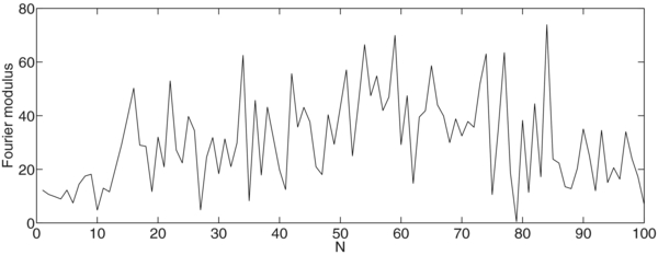
Figure 7. Fourier transform of the frequency spectrum (after subtraction of its smoothed frequency spectrum) of a typical galaxy that did not produce a signal.
Download figure:
Standard image High-resolution image
Figure 8. Spectrum of the galaxy in Figure 7, in frequency units, after subtraction of the smoothed continuum. The spectrum was blueshifted to a redshift z = 0.0 to facilitate a comparison with Figures 6 and 11.
Download figure:
Standard image High-resolution imageThe similarities among the spectra of galaxies both with detected signals and those with undetected signals leads to the conclusion that the signal is not caused by the Fourier transform of spectral lines. The computer simulations discussed in the next section quantitatively elaborate on this statement.
5. COMPUTER SIMULATIONS
The discussion in the previous section concludes that the signals are not due to the Fourier transform of the spectral lines, but this conclusion is mostly qualitative. This section presents the results of computer simulations that strengthen this conclusion.
The sharp peak seen in Figure 2 is typical of the peaks detected in the objects that are plotted in Figure 3. It looks like a Kronecker delta function. However, because it is the result of the Fourier transform of a spectrum, it cannot be a delta function because a delta function would be the result of the Fourier transform of the entire spectrum and would be centered at N = 0. This peak could, however, be the tooth of a comb-like function that we can conveniently model with a Shah function because the Fourier transform of a Shah function III(f−nF) (where n is an integer number and F is the period of variation in frequency units) in the frequency domain f gives another Shah function III(t−n/F) having a period P = 1/F in the time domain t. We can therefore model the absorption lines in the frequency spectrum I(f) of a galaxy by the convolution of a Shah function with a Gaussian function that conveniently models a line profile. The Fourier transform of a convolution is the product of the Fourier transforms of the two functions. The Fourier transform of a Gaussian with a dispersion σ is another Gaussian with a dispersion ∼1/σ. Consequently, the Fourier transform of a spectrum I(f) with periodically recurrent spectral lines, modeled by a Shah function III(f−nF) with period F, convolved with a Gaussian function with a dispersion σ, is another Shah function III(t−n/F) with a period P = 1/F multiplied by a Gaussian with a dispersion ∼1/σ centered at N = 0.
Starting from the analytical discussion in the previous paragraph, we have carried out numerical simulations using Matlab software that model an SDSS spectrum in the frequency domain with a flat continuum from which one subtracts the convolution of the Shah function with a Gaussian to simulate a spectrum that contains absorption lines. Because the time shown in Figure 2 is T = 1.13 × 10⁻¹³ s and the Fourier transform of the Shah function gives a frequency period F = 1/T = 8.45 × 10¹² Hz, the frequency spectrum must contain spectral lines separated by 8.45 × 10¹² Hz. Figure 9 shows the result of the FFT of a spectrum that uses this model. The dispersion of the Gaussian function used to simulate the absorption lines was obtained from the average width of the absorption lines in the spectrum of the galaxies in Figures 6 and 8, which is typical of the width of the lines in a typical galaxy observed in the SDSS survey. The fact that we approximate the spectral line of a galaxy with a Gaussian only causes the minor error that the Shah function III(t−n/F) is multiplied by the Fourier transform of a Gaussian instead of the Fourier transform of the exact shape of the spectral line. Because both of these functions have the same half-widths, we can understand that the approximation has a minor effect. Figure 9 confirms the theoretical discussion based on the Shah function in the previous paragraph. However, it is obviously not in agreement with Figure 1, since Figure 1 only shows one peak. On the basis of Figure 9, we would have expected three visible peaks, even considering the presence of noise. Furthermore, the numerical frequency spectrum that generates Figure 9 contains 50 spectral lines equally spaced by 8.45 × 10¹² Hz and having equal peak intensities = −0.6 in the smoothed spectrum, which is in obvious disagreement with the spectrum in Figure 6.
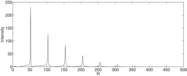
Figure 9. Fast Fourier transform of a Shah function convolved with a Gaussian.
Download figure:
Standard image High-resolution imageTo understand the effect of changing the intensities of the absorption lines as well as their frequency locations, more simulations were carried out. These simulations used the same basic spectrum of the convolution of the Shah function with a Gaussian that generated Figure 9, but added Matlab code that changed at random the intensities and frequency locations of the individual lines. The intensity of the lines was changed by multiplying the peak intensity of every line with the Matlab function "rand" that generates random numbers having values uniformly distributed between 0 and 1. The frequency locations of the absorption lines were also changed with rand multiplied by a constant smaller than one and by the equal frequency separation of 8.45 × 10¹² Hz in the Shah function. Such a random frequency location shift generated by rand was then added to the frequency position of the Shah function. A different frequency deviation from the periodic frequency location predicted by the Shah function was therefore randomly generated for every one of the periodic 50 frequency locations of the absorption lines. After several simulations, we found that a signal similar to the signal seen in Figure 2 could be generated with appropriate values of the constant that multiplies rand. Figure 10 shows an example of such a simulation. A strong peak, similar to the one in Figure 2, can clearly be seen. At first glance, this result seems to confirm the hypothesis; however, in practice, this result does not because too many strong lines at the appropriate peculiar frequency locations are required. We elaborate on this topic in the next paragraphs.

Figure 10. Fast Fourier transform of a simulation that used the same basic spectrum of the convolution of the Shah function with a Gaussian that generated Figure 9, but with a computer code that changed at random the intensities of the lines (from 0.0 to −0.7) and the frequency locations of the individual lines (−0.1% average deviation from the Shah function frequency positions).
Download figure:
Standard image High-resolution imageFigure 11 shows the frequency spectrum that was used to generate Figure 10 with a Fourier transform. The intensities of the lines were chosen to produce a signal equal to the signal seen in Figures 1 and 2; consequently, this spectrum can be readily compared to the spectrum in Figure 6 as well as the spectrum in Figure 8. The positions of the lines have the periodicity (in frequency units) required to produce the peak seen in Figure 10, but have an additional random deviation from that value generated with the function rand (see previous paragraph). The average deviation from the 8.45 × 10¹² Hz frequency period is ±7.5%, which corresponds to a ±0.1% deviation from the periodic frequency position, so that the positions of the spectral lines are still reasonably periodic in frequency. A comparison of Figure 11 with Figures 6 and 8 shows that a large number of absorption lines strong enough to be seen with visual inspection should be present in Figure 6 but not in Figure 8. Of course, one does not need to add 50 spectral lines to the spectrum of Figure 8 to generate, after the Fourier transform, a signal similar to the signal seen in Figure 2. First, some of the lines in Figure 11 are weak and would not be detectable in a visual inspection of Figures 6 and 8. Second, because one would need to add lines to the spectrum of Figure 8, some of the lines in that spectrum would presumably already be near the needed location and one would therefore have to add a number fewer than 50. Note that Figure 8 could only have a very small number of lines at the required frequencies; otherwise, they would have generated a visible peak in Figure 7. A comparison of Figures 6, 8, and 11 therefore clearly shows that significant numbers of lines detectable with visual inspection would have to be added to Figure 8 to generate a peak similar to the peak visible in Figure 2. Half of the lines in Figure 11 have an intensity equal to or stronger than −0.4 and therefore should be easily detectable in Figures 6 and 8. In conclusion, because Figures 6 and 8 are so similar, we can exclude that the required number of additional lines are present in Figure 6.

Figure 11. Frequency spectrum used to generate Figure 10 with a Fourier transform.
Download figure:
Standard image High-resolution image
Note that the total number of required strong lines seen in the theoretical Figure 11 is about the same total number of lines visible in the spectra in Figures 6 and 8. Finally, the required lines must be present in a continuous spectral region that is at least 70% of the total spectrum, otherwise, after the Fourier transform, the peak would be broader than what is seen in Figure 10 with a width inversely proportional to the width of the region that contains the lines. For example, if the periodic lines are only present in the left half of the spectrum (between 320 THz and 550 THz) and not the right half, the peak in Figure 2 would have been two samples wide (ΔN = 2) instead of one (ΔN = 1). If the lines are only present in a region having a width equal to 1/4 of the spectrum, the peak would have been four samples wide (ΔN = 4).
The hypothetical lines that would generate the signal must be among the strongest in the spectra. This result can be seen by comparing the numerical simulation figures to the observational figures. This fact can also be seen in the Fourier transform domain. Figure 10, generated by the FFT of Figure 11, shows that the average Fourier "continuum" generated by the FFT of the lines is strong because it has an amplitude of 50, half the amplitude of 100 of the Fourier "continuum" of the detected galaxy in Figure 1. However, the numerical Fourier spectrum in Figure 10 does not include the effects of random noise. The standard deviation due to random noise in Figures 1 and 2 is equal to eight; therefore, to estimate the contribution of noise, one must add to the numerical Figure 10 a noise contribution with an upper limit of about 24, equal to three standard deviations. This procedure produces an amplitude of 80, comparable to the Fourier continuum amplitude in Figure 2.
6. DISCUSSION AND CONCLUSION
A statistically significant signal has been found in a very small fraction of the galaxies observed (223 out of 0.9 million) for a signal-to-noise ratio >6.5. No signal was detected at these N locations in over 0.5 million stars and quasars observed. All evidence is consistent with a signal coming from a periodic modulation of the frequency spectrum. The tight redshift dependences shown in Figures 3 and 4 and the fact that neither a single star nor a single quasar was detected exclude the possibility of instrumental effects. Computer simulations show that the signal shown in Figures 1 and 2 implies a periodic modulation, like in Equation (5) in Borra (2010), with amplitude ± 0.2 in its frequency spectrum in Figure 6. At this amplitude, the signal is buried in the noise in Figure 6 such that one would not expect to see it with a simple visual inspection.
The hypothesis that the signal is caused by the Fourier transform of spectral lines, discussed in Sections 5 and 6, is not in agreement with the observational evidence because the spectra of galaxies that have the signal and the spectra of those that do not have it are too similar. In reading the discussions in Sections 5 and 6, one has to consider that the SDSS spectra of the galaxies have low spectral resolution and low signal-to-noise ratios. Consequently, to produce a signal after the FFT of an SDSS spectrum, the spectral lines would have to be strong. Besides the observational evidence, other arguments also go against the hypothesis. In principle, large differences in stellar type distributions may do the job. However, there is no justifiable reason that adding different spectral types would produce the needed periodic frequency modulation. The FFTs of the spectra of late spectral type stars, which are more representative of the spectra of galaxies, do not show any significant peaks at all. The only stars that have significant peaks are early-type stars and their peaks are not located at N = 52 as required. Note also that the detected galaxies have a single peak (see Figures 1 and 2), while the FFTs of A and B stars have two broad peaks with the main peak at N = 37 and a weaker peak at N = 57 (see Figure 5), while O stars have the main peak at N = 45 and a weaker peak at N = 62. Adding more lines at the required frequencies would narrow the widths of the Fourier peaks, but would not change their locations. Another possibility comes from differences in chemical abundances. However, there is no obvious evidence that changing chemical compositions would produce additional lines at the required spectral locations. Because the hypothetical lines are absorption lines in the spectra of galaxies, this hypothesis would imply large peculiar chemical compositions in a large fraction of stars. Intuitively, the hypothesis of highly peculiar chemical abundances may be credible for a single star but, on the basis of what we know about chemical abundances in the universe, it seems highly unlikely that the large fraction of stars needed in a galaxy would have strong, very peculiar chemical compositions. Note also that simply increasing the known chemical compositions of galaxies would not do the job because the Fourier spectra of the undetected galaxies do not show any evidence of a weak peak (see Figure 7). Furthermore, the number of detected galaxies is very small and decreasing the signal-to-noise ratio criterion increases the number of detections below the number expected from Rayleigh statistics (see Section 3). Another major problem with the FFT of the spectral line hypothesis comes from the fact that, in Figures 3 and 4, the positions of the signals increase linearly with redshift along two linear staircases that have different bases (for a redshift z = 0.0) at N = 52 (1.09 × 10⁻¹³ s) and N = 49 (1.03 × 10⁻¹³ s). Consequently, one would need two sets of galaxies having spectral lines positioned at two slightly different frequency periods and therefore two different types of highly peculiar chemical abundances. This fact renders the hypothesis even less credible, especially considering that we are dealing with the spectra of galaxies and not with the spectra of single stars. It must be noted that even if turns out that the signal is due to the Fourier transform of the spectral lines, this would be an interesting discovery because it would imply the existence of a small number of galaxies with highly peculiar chemical compositions. An obvious question that arises is: what is the fundamental reason why spectral lines in the simulations generate a signal similar to a cosinusoidal modulation? The answer is that the signal that is added comes from spectral lines that are positioned at periodically recurrent positions so that we can model the signal with a cosinusoidal curve.
At this stage, one can only speculate on the physics responsible for the spectral modulation, as we do in the following paragraphs.
As discussed in Section 3, decreasing the signal-to-noise threshold to 6.0 from 6.5 for the entire survey would have increased the number of detected galaxies by a factor of 7.4 (from 223 to 1660), while Rayleigh statistics predict a factor of 23. The fact that the detections are significantly below those predicted by Rayleigh statistics, which apply to our detections because we use the Fourier modulus, indicates that the signals are strong signals that come from a very small fraction of galaxies. This result is consistent with signals coming from strong light beams present in many galaxies but detected in only a few of them because the beams have small divergences. This situation is what one intuitively expects from non-thermal sources that produce a jet. This result would also arise from the kind of beam seen in pulsars.
The signal could be generated by sources sending pulses separated by times of the order of 10−13 s, which was the original principal reason for searching for spectral periodicities (Borra 2010). However, at this stage, this idea is only a hypothesis to be verified with further work. One may object that to generate pulses separated by 10−13 s would necessitate very small volumes having absurdly large implied brightness temperatures. As an answer to this objection, one can note that the extreme unresolved (<0.5 ns) pulses of the Crab pulsar have a similar problem resulting in an implied brightness temperature of 2 × 1041 K (Hankins & Eilek 2007). Borra (2010) elaborates on this subject. Furthermore, the radio spectrum of the Crab pulsar also shows spectral bands (Hankins & Eilek 2007) that show the type of spectral modulation that has been detected in galaxies, although the spacing between the radio bands increases linearly with frequency instead of being constant. This result may possibly due to the effect of the pulsar environment since electromagnetic waves at radio frequencies are affected by the high-energy ionized environments they flow through.
On the one hand, the strong relationship seen in Figures 3 and 4, which implies that the period is constant in the reference frame of the galaxies, clearly indicates the presence of a puzzling effect. On the other hand, this relationship places severe constraints on the physics responsible. Because galaxies have a central massive black hole, unknown exotic physics may be responsible. Other explanations are also obviously possible.
Some galaxies were observed on different Julian dates. Some were detected (e.g., the galaxy in Figure 1), albeit with a lower signal-to-noise ratio, but some were not. This result may be due to variability but also the effect of random noise.
The detected objects will have to be observed again to confirm the effect in spectra with high signal-to-noise ratios. A list of the objects can be found in Trottier (2012) and will be published in a forthcoming paper. We will also provide these data upon request.
This research has been supported by the Natural Sciences and Engineering Research Council of Canada. The author thanks Eric Trottier for the remarkable work he performed analyzing the SDSS data. Funding for SDSS-III has been provided by the Alfred P. Sloan Foundation, the Participating Institutions, the National Science Foundation, and the U.S. Department of Energy Office of Science. The SDSS-III website is http://www.sdss3.org/.