A MEGACAM SURVEY OF OUTER HALO SATELLITES. II. BLUE STRAGGLERS IN THE LOWEST STELLAR DENSITY SYSTEMS*

Felipe A. Santana; Ricardo R. Muñoz; Marla Geha; Patrick Côté; Peter Stetson; Joshua D. Simon; S. G. Djorgovski

doi:10.1088/0004-637X/774/2/106

1. INTRODUCTION

Blue stragglers are stars coeval with a given stellar population, but positioned blueward and above its main-sequence turnoff (MSTO), thus mimicking a younger population. They were first observed by Sandage (1953) in the globular cluster (GC) M3 as an apparent extension of the classical main sequence (MS; see, for example, Bailyn 1995 for a review on blue stragglers). Since globular clusters have traditionally been considered single stellar populations, stars located blueward and above the MSTO in their color–magnitude diagrams (CMDs) should have evolved off of the MS into a post hydrogen-burning phase. In this context, the existence of blue straggler stars challenges our current understanding of stellar evolution. To inhabit a hotter and more luminous region of the CMD, these stars must have increased their original masses and, in the process, renewed their fuel for nuclear reactions.

Since the discovery made by Sandage, blue stragglers have been found in practically all Galactic globular clusters, and several formation mechanisms have been proposed. Early on, blue stragglers as single stars were proposed, either massive young stars due to recent star formation, or stars in a post-helium flash evolutionary phase where hydrogen-rich material has sunk to the core (Rood 1970; Conti et al. 1974). These formation mechanism were, however, later discarded (e.g., Nemec & Harris 1987; Nemec & Cohen 1989). At present, the leading blue straggler star formation mechanisms are stellar mergers produced by direct stellar collisions (hereafter collisional blue stragglers, e.g., Hills & Day 1976; Leonard 1989) and mass-transfer or mergers in primordial binary or higher-order systems (hereafter binary blue stragglers, e.g., McCrea 1964; Knigge et al. 2009; Perets & Fabrycky 2009). Several studies have used photometric variability to show that some blue stragglers are indeed binary systems (Jorgensen & Hansen 1984; Mateo et al. 1990, 1995; Nemec et al. 1995). On the other hand, triples have been claimed to be particularly relevant in blue straggler formation in low-density environments (Leigh & Sills 2011). Triples could form blue stragglers through mechanisms like Kozai cycles and tidal friction (Perets & Fabrycky 2009) or triple evolution dynamical instabilities (Perets & Kratter 2012). The importance of collisions involving triple stars in forming blue stragglers was confirmed by Geller et al. (2013) through N-body modeling of the old open cluster NGC 188. Bailyn (1995) argued that both mechanisms (binary and direct collisions) are likely to be at work in globular clusters, a view shared by several studies (e.g., Hurley et al. 2001; Mapelli et al. 2006; Dalessandro et al. 2008; Ferraro et al. 2009). The relative importance of these two mechanisms is a function of cluster mass (Davies et al. 2004) and the dynamical evolution and physical conditions of the environment (Piotto et al. 2004; Knigge et al. 2009; Leigh et al. 2011b).

To investigate the relative importance of the two formation mechanisms, several correlations between the observed fraction of blue straggler stars and host properties have been explored. For example, the fraction of blue stragglers can be plotted as a function of density or encounter rate. If the fraction of blue stragglers grows with density, then collisions might be the dominant formation mechanism. If instead we find fewer blue stragglers in denser systems, collisions between stars might prevent blue straggler formation, either by separating primordial binaries or by disrupting multiple star systems. Perhaps the most notable result in this context was reported by Piotto et al. (2004), who found that the blue straggler specific fraction declines with increasing luminosity or mass. The interpretation of this anti-correlation is that the current fraction of binary stars, from which blue stragglers would form, would be lower for larger and denser systems (Leigh et al. 2011b; Sollima et al. 2008; Davies et al. 2004). Although, in the magnitude range spanned by Piotto's globular cluster sample, −10 < M_V < −6, a significant contribution from collisionally formed blue straggler stars cannot be discarded.

In addition to globular clusters, blue stragglers have been detected in a variety of low-density environments such as Galactic dwarf spheroidal (dSph) galaxies (e.g., Momany et al. 2007), loose stellar clusters (e.g., Geller & Mathieu 2011; Sollima et al. 2008), the Milky Way's bulge (Clarkson et al. 2011), and even the Galactic field (e.g., Stetson 1991; Glaspey et al. 1994; Preston & Sneden 2000; Carney et al. 2001, 2005). Currently, the number of studies of blue stragglers in dSph galaxies is rather limited, and in most cases they cover only one or two galaxies (see Mapelli et al. 2007 for Draco and Ursa Minor, Hurley-Keller et al. 1999 and Monkiewicz et al. 1999 for Sculptor, and Mateo et al. 1995 for Sextans). Only one study to date presents a systematic study among classical dSph galaxies (Momany et al. 2007).

On the other hand, information regarding blue straggler stars in ultra-faint dwarf (UFD) galaxies is extremely scarce with only a couple of studies mentioning the potential presence of blue stragglers in UFDs (Martin et al. 2008a; Sand et al. 2010). The UFDs correspond to a recent population of dark matter-dominated satellites found in the Milky Way halo as stellar overdensities in the Sloan Digital Sky Survey (SDSS) photometric catalog (e.g., Willman et al. 2005b; Belokurov et al. 2006, 2007, 2010; Zucker et al. 2006; Irwin et al. 2007), with total luminosities even lower than those of the previously known dSphs, ranging from M_V ∼ −8 down to M_V = −1.5 for the faintest system yet found (Segue 1). These extreme low luminosity, low surface brightness systems represent a new opportunity to study blue straggler stars in extremely low stellar density environments.

In this study, we use a new survey carried out with the Canada–France–Hawaii Telescope (CFHT; R. R. Muñoz, in preparation). This survey is aimed at obtaining wide-field photometry of all bound stellar overdensities in the outer halo (i.e., with Galactocentric distances greater than 25 kpc). Here, we present a homogeneous analysis of the blue straggler star populations of most of these Milky Way halo satellites, to study the characteristics of blue straggler stars in the lowest stellar density systems. The analysis includes globular clusters, dSphs, as well as the first systematic study of blue stragglers in the UFDs.

Collisions involving single, binary, or triple stars are not likely to occur in our systems. The expected time for this type of interactions to occur are large compared to the blue straggler lifetime. Therefore, except for a few of our highest density systems, the blue stragglers in our Galactic satellites might not be explained by collisions of any type. Moreover, the densest objects in our sample, the outer halo clusters, are, as a group, fainter and on average 10 times bigger than their inner halo counterparts. Our goal is to investigate the presence/absence of blue straggler stars in the most diffuse stellar systems and to study the influence of the environment on their blue straggler star populations. This paper is organized as follows: in Section 2, we describe the photometric catalog and the sample of satellites used in this study. We also detail how blue straggler stars are selected and how their counts are normalized to red giant branch (RGB) stars. In Section 3, we present our results, including modeling of young populations that could be mimicking blue straggler stars in dwarf galaxies. In Section 4, we discuss our results for each type of satellite. Finally, a brief summary is presented in Section 5.

2. DATA AND BLUE STRAGGLER SELECTION

We analyzed the blue straggler star population of 22 outer halo (beyond R_G = 25 kpc) satellites: 10 globular clusters, 3 of the classical dSph galaxies (Draco, Ursa Minor and Sextans), and 9 UFDs. Data for all objects were obtained using the CFHT MegaCam imager; these data represent a subsample of a larger program aimed at obtaining wide-field photometry of all bound stellar overdensities in the outer halo (R. R. Muñoz et al., in preparation). The first results from this survey were presented in Muñoz et al. (2012a), who reported the discovery of a very low luminosity star cluster at a distance of ∼45 kpc along the line of sight to the Ursa Minor dSph galaxy. From the entire sample of objects in this survey, the 22 systems considered here correspond to the ones where blue straggler stars could be reliably selected in the CMD. In the excluded systems, extreme low star counts, severe overcrowding, or photometry issues prevented a robust blue straggler discrimination, and would have added large systematic errors to the analysis.

For each system, six dithered exposures in the CFHT g- and r-bands were taken in mostly dark conditions. A standard dithering pattern was chosen from the MegaCam operation options to cover all gaps between chips. The exposure times varied between objects, but in all cases reached at least 1 mag below the MSTO of the satellite. Details of the observing log (i.e., exposure time, seeing conditions, etc.) will be given elsewhere.

Data from MegaCam were pre-processed prior to release using the "ELIXIR" package (Magnier & Cuillandre 2004), which includes bias subtraction, flat fielding, bad pixel correction and preliminary solutions for photometry and astrometry. We carried out subsequent data analysis using the DAOPHOT/Allstar/ALLFRAME package (Stetson 1994), following the method detailed in Muñoz et al. (2010). To remove non-stellar objects and spurious detections, we used the DAOPHOT Chi and sharp parameters. We selected sources with Chi < 5 and −0.4 < sharp < 0.4. In addition, we only used detections with photometric uncertainties smaller than 0.1 mag in both bands. Finally, we calibrated our observations using SDSS data, which allowed us to obtain our final calibrated magnitudes translated into SDSS g- and r-bands. We note that overcrowding affects only a few objects since most outer halo clusters are, on average, more extended and less luminous than their inner halo counterparts, and therefore have lower stellar densities. In the cases where overcrowding could have been a problem, completeness at the magnitude of the MSTO was larger than 50% in the entire system with the exception of the very central region. The areas of these regions were in all cases more than a factor of 30 smaller than the total area of the system. Therefore, even for these systems, overcrowding produces a negligible effect on our results. In Figure 1, we show the CMDs of all the sources selected as stars for different globular clusters, classical dwarf galaxies, and UFD galaxies in our sample.

**Figure 1.** M_g vs. (g − r) extinction corrected color–magnitude diagrams of stars in nine different satellites from our sample, obtained at the Canada–France–Hawaii Telescope. Classical dwarf galaxies are shown in the top panels, UFD galaxies are shown in the middle panels, and three of the globular clusters in our sample are shown in the bottom panels. Boxes where blue straggler and red giant branch stars were counted are shown for each case.
Download figure:
Standard image High-resolution image

To select blue straggler stars, we defined a box in the dereddened (g − r) versus M_g diagram of each object. The size and shape of this box was chosen to maximize the blue straggler counts while at the same time minimize contaminants from other stellar populations. We determined the distance from the blue straggler box to the MSTO position based on typical MS widths and photometric uncertainties. Likewise, the bright side of the blue straggler box was chosen based on typical blue horizontal branch extensions. In Figure 2, we show our blue straggler star selection criteria for the UFD galaxy Boötes I as an illustration. The coordinates of the four points in the CMD that define the blue straggler star⁶ box for each object, relative to the MSTO position, had typical [Δ(g − r),ΔM_g] values of (−0.245,−0.405), (−0.554,−1.969), (−0.362,−3.012), and (−0.010, −1.513). Small shifts, with typical values of 0.015 in color and 0.09 in magnitude, were applied in some objects to move the entire box. These shifts are mainly caused by uncertainties in the position of the MSTO and our intention, in certain objects, of avoiding regions significantly contaminated. Varying the bright and dim side of our blue straggler box, along with applying the shifts, does not significantly change our results since these variations are shown to be small compared to our random errors.

**Figure 2.** Stars in the Boötes I field. Left: Boötes I M_g vs. (g − r) extinction-corrected color–magnitude diagram. Blue and red lines show, respectively, Padova isochrones of 1 and 12 Gyr, with a metallicity of [Fe/H] = −2.1. The blue box shows the color–magnitude diagram region were blue straggler stars were counted, while the RGB region is delimited by the red box. Stars considered as blue stragglers are shown as blue squares. Right: star map of the Boötes I UFD. The blue curve shows the limit for the system region at twice the half-light radius, while the red annuli show the limits for the contamination region, at five and six times the half-light radius, respectively.
Download figure:
Standard image High-resolution image

The data were dereddened for all satellites using values for E(B − V) taken from Schlegel et al. (1998). These values were translated into Sloan filter extinctions A_g and A_r, using the transformations of Schlafly & Finkbeiner (2011). Absolute magnitudes were derived using distance values from the literature.⁷ We derived metallicities by fitting Padova isochrones to the main old population.

To compare the number of blue straggler stars among systems with different absolute magnitudes, a common practice (e.g., Piotto et al. 2004; Leigh et al. 2007) is to normalize the blue straggler star counts to those of another subpopulation, typically RGB or blue horizontal branch stars. For this study, we chose RGB stars since they are more numerous than blue horizontal branch stars. This choice reduces shot noise due to the low number of stars, a problem especially critical for the UFDs (Martin et al. 2008b; Muñoz et al. 2012b). To avoid introducing a significant bias when using RGB stars as a normalization population, we checked that the number of these stars grows linearly with luminosity. Figure 3 shows that RGB star counts are indeed proportional to the flux of the systems, with a correlation factor of r² = 0.91, confirming that RGB stars are good tracers of total stellar luminosity or mass. To select RGB stars, we defined a box centered on a 12 Gyr old Padova isochrone (with the appropriate metallicity for each system), 0.19 mag wide and located between 2.4 and 4.9 mag below the RGB tip. To count both blue straggler and RGB stars, we used an elliptical region within two times the half-light radius (r_h) of the system. For each case, this region was defined by the ellipticity and position angle derived in R. R. Muñoz et al. (in preparation), based on the same CFHT data. To account for background/foreground contaminants, we counted sources in both the blue straggler and RGB boxes, but in annuli at distances greater than 4 × r_h from the center of the object. An example is shown in the right panel of Figure 2 and the values of the inner and outer annuli of the contamination region, in terms of r_h, are shown in Table 1 for each object.

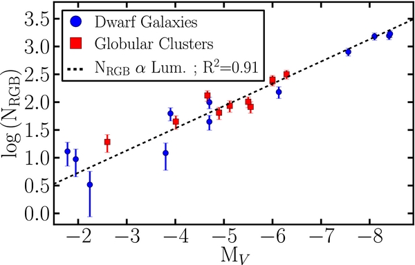
**Figure 3.** Red giant branch star numbers plotted against the absolute magnitude of each system. The figure shows that our normalization population numbers are directly proportional to the total luminosity of the system. Dashed black line shows a linear relation between luminosity and red giant branch star counts; the data have a correlation factor of 0.91.
Download figure:
Standard image High-resolution image

Table 1. Blue Straggler Stars and RGB Counts for All Satellites

Object	Type	BSS_T^a	Norm BSS_C^b	RGB_T^c	Norm RGB_C^d	$F_{\rm {RGB}}^{\rm {BSS}}$ ^e	n_rh (stars pc^-3)^f	$\frac{r_{\rm {cont,inn}}}{r_{\rm {half}}}$ ^g	$\frac{r_{\rm {cont,out}}}{r_{\rm {half}}}$ ^h
Boötes I	UFD	71	16.19	230	77.73	0.36 ± 0.07	2.1 × 10⁻³	5.0	6.0
Boötes II	UFD	4	1.20	18	5.00	0.26 ± 0.17	5.9 × 10⁻³	4.0	6.0
Coma Berenices	UFD	10	4.00	21	8.83	0.49 ± 0.33	4.6 × 10⁻³	5.0	7.0
Canes Venatici I	UFD	343	91.98	842	40.37	0.31 ± 0.03	6.0 × 10⁻⁴	4.8	5.8
Hercules	UFD	35	9.43	127	27.57	0.26 ± 0.07	4.1 × 10⁻⁴	6.0	8.0
Segue 2	UFD	3	0.60	13	3.57	0.26 ± 0.22	7.4 × 10⁻³	5.0	6.2
Ursa Major I	UFD	19	6.36	56	11.59	0.28 ± 0.12	3.8 × 10⁻⁴	5.5	7.0
Ursa Major II	UFD	23	3.85	79	16.42	0.31 ± 0.09	1.2 × 10⁻³	5.0	7.0
Willman 1	UFD	3	0.21	4	0.72	0.85 ± 0.75	2.2 × 10⁻²	5.0	8.0
Draco	dSph	422	17.82	1600	76.73	0.27 ± 0.02	1.2 × 10⁻²	5.0	6.0
Sextans	dSph	521	65.49	1822	260.35	0.29 ± 0.02	1.3 × 10⁻³	4.0	5.0
Ursa Minor	dSph	514	14.00	1743	47.36	0.30 ± 0.02	3.3 × 10⁻³	5.0	6.5
NGC 5694	GC	11	0.15	247	6.97	0.05 ± 0.01	7.5 × 10⁰	15.0	19.0
NGC 6229	GC	11	0.19	318	1.66	0.03 ± 0.01	1.5 × 10¹	14.0	18.0
NGC 7006	GC	19	0.12	263	9.06	0.07 ± 0.02	6.1 × 10⁰	14.0	18.0
NGC 7492	GC	8	0.08	83	0.75	0.10 ± 0.04	1.4 × 10¹	16.0	20.0
Eridanus	GC	12	0.25	45	0.39	0.26 ± 0.09	2.7 × 10⁻¹	20.0	28.0
Palomar 3	GC	11	0.15	65	0.44	0.17 ± 0.06	8.5 × 10⁻¹	20.0	30.0
Palomar 4	GC	10	0.12	102	0.44	0.10 ± 0.03	1.5 × 10⁰	20.0	30.0
Palomar 13	GC	8	0.12	20	0.75	0.41 ± 0.18	1.4 × 10⁰	16.0	22.0
Palomar 14	GC	15	0.75	91	5.14	0.17 ± 0.05	1.6 × 10⁻¹	12.0	16.0
Palomar 15	GC	20	1.32	150	18.25	0.14 ± 0.04	6.5 × 10⁻¹	12.0	16.0

Notes. ^aBlue straggler stars measured in the system region. ^bBlue straggler stars measured in the contamination region normalized by area. ^cRGB stars measured in the system region. ^dRGB stars measured in the contamination region normalized by area. ^eSpecific fraction of blue stragglers as measured from Equation (1). ^fStellar density measured within the half-light radius of the system. ^gInner radius of contamination region normalized to the half-light radius. ^hOuter radius of contamination region normalized to the half-light radius.

Download table as: ASCII Typeset image

Once blue stragglers, RGB stars, and contamination objects were selected, we defined the specific fraction of blue stragglers as:

$\begin{equation} F_{\rm {RGB}}^{\rm {BSS}}=\frac{{\rm BSS}_{\rm {s}}-{\rm BSS}_{\rm {c}}}{{\rm RGB}_{\rm {s}}-{\rm RGB}_{\rm {c}}}, \end{equation} \tag{ 1 }$

where BSS means "blue straggler star" and the subscripts s and c correspond to "system" and "contamination," respectively.

3. RESULTS

3.1. Blue Straggler Specific Fractions

In Table 1, we list the resulting blue straggler and RGB star counts, along with the corresponding blue straggler specific fractions, limits for the contamination region, and the density of our clusters and galaxies.

A surprising first result is that blue stragglers seem to be ubiquitous among dwarf galaxies, being present even in the most diffuse and least luminous systems. In Figure 4, we plot $F_{\rm {RGB}}^{\rm {BSS}}$ against absolute magnitude, M_V. This figure shows that the blue straggler star fraction distribution for galaxies is statistically consistent with being flat over a 6 mag range, with a weighted mean value of:

$\begin{equation} \left. \overline{F_{\rm {RGB}}^{\rm {BSS}}}\right| \rm {_{dwarfs}} = 0.29\pm 0.01 \end{equation} \tag{ 2 }$

and a standard deviation of 0.17. In contrast, for globular clusters, we see a well-defined anti-correlation between $\log ({F_{\rm {RGB}}^{\rm {BSS}}})$ and the absolute magnitude of the objects. The linear function fitted has the form:

$\begin{equation} \left. \log \left({F_{\rm {RGB}}^{\rm {BSS}}} \right)\right|{\rm _{clusters}} = (0.28\pm 0.04) M_{\rm V} + (0.50\pm 0.22). \end{equation} \tag{ 3 }$

The uncertainties in the fitting parameters of this and all the forthcoming equations were estimated using Monte Carlo simulations. Each time we ran a simulation, we shifted the data by values consistent with the uncertainties in the measured frequencies and then calculated the set of fitting parameters that corresponded to that shifted data sample. Then, for each fitting parameter, the uncertainty was determined to be the standard deviation of the values obtained in the different runs.

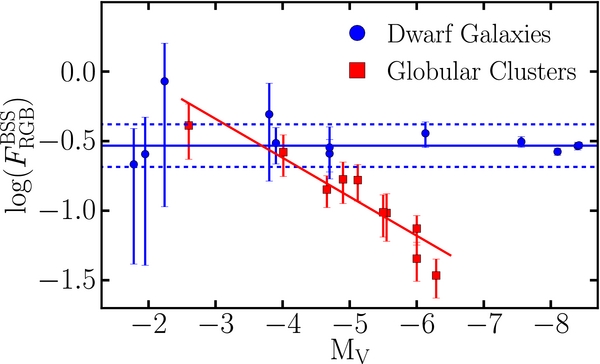
**Figure 4.** Specific fraction of blue stragglers $F_{\rm {RGB}}^{\rm {BSS}}$ plotted against absolute magnitude. A clear anti-correlation can be seen for clusters, while dwarf galaxies show a high and flat distribution. The logarithm of the weighted mean of ${F_{\rm {RGB}}^{\rm {BSS}}}$ is shown as a solid blue line while dashed blue lines show the standard deviation around this value. The red solid line shows the fit for clusters corresponding to $\log ({F_{\rm {RGB}}^{\rm {BSS}}})$ ∝ (0.28 ± 0.04) *M_V*.
Download figure:
Standard image High-resolution image

**Figure 4.** Specific fraction of blue stragglers $F_{\rm {RGB}}^{\rm {BSS}}$ plotted against absolute magnitude. A clear anti-correlation can be seen for clusters, while dwarf galaxies show a high and flat distribution. The logarithm of the weighted mean of ${F_{\rm {RGB}}^{\rm {BSS}}}$ is shown as a solid blue line while dashed blue lines show the standard deviation around this value. The red solid line shows the fit for clusters corresponding to $\log ({F_{\rm {RGB}}^{\rm {BSS}}})$ ∝ (0.28 ± 0.04) *M_V*.
Download figure:
Standard image High-resolution image

This result is consistent with a similar anti-correlation found by Piotto et al. (2004) for a group of 56 globular clusters, most of them in the inner halo. In our study, however, we have expanded the anti-correlation to clusters that are 3 mag fainter. Even though we used RGB stars as a normalization population and horizontal branch stars were used in Piotto et al. (2004), the slopes of the anti-correlations found in both studies are consistent within the errors.

A different normalization method (first outlined in Knigge et al. 2009) was also used to illustrate the dependence of blue straggler population sizes on the total population size of their hosts. As seen in Figure 5, we correlated the number of blue stragglers observed with the total stellar mass of our systems. The linear fitting functions we obtained using this normalization were:

$\begin{eqnarray} \log {(N_{\rm {BSS}})} &=& (0.06\pm 0.07) \log {(\rm {Mass})} + (0.8\pm 0.3) \nonumber\\ && \quad \hbox{(for globular clusters)} \end{eqnarray} \tag{ 4 }$

$\begin{eqnarray} \log {(N_{\rm {BSS}})} &=& (0.90\pm 0.04) \log {(\rm {Mass})} + (-2.4\pm 0.2) \nonumber\\ && \quad \hbox{(for dwarf galaxies).} \end{eqnarray} \tag{ 5 }$

Both correlations found here are equivalent to the results found before using the specific frequency of blue stragglers. Blue straggler numbers in clusters increasing slowly with mass is equivalent to an anti-correlation of $F_{\rm {RGB}}^{\rm {BSS}}$ and M_V like the one in Equation (3). On the other hand, blue straggler numbers in dwarf galaxies growing almost linearly with mass is equivalent to a nearly constant distribution of $F_{\rm {RGB}}^{\rm {BSS}}$ . Within the errors, Equations (2) and (5) point to specific blue straggler fractions in dwarfs that are either independent of absolute magnitude or follow a shallow anti-correlation with absolute magnitude like the one found by Momany et al. (2007).

**Figure 5.** The number of blue stragglers plotted against the total stellar mass of each system. The fitting function for clusters is log (N_BSS) ∝ (0.06 ± 0.07) log (M) and is shown as a red line. The fitting function for galaxies is log (N_BSS) ∝ (0.90 ± 0.04) log (M) and is shown as a blue line.
Download figure:
Standard image High-resolution image

Finally, we plot blue straggler specific frequencies against both the density within r_h (see Figure 6) and the encounter rate between single–single stars (see Figure 7), as calculated in Leigh & Sills (2011). Figure 6 shows that blue straggler frequencies of all our systems follow a single exponential trend with density, displaying a smooth transition between clusters and galaxies. Figure 7, on the other hand, shows that the same behavior is followed by the frequency of blue stragglers versus the encounter rate. The fraction of blue stragglers stays constant and high in the low-density/low encounter rate regime spanned by our dwarf galaxies and decreases with density and encounter rate in the range spanned by our globular clusters. The fitting functions that describe the blue straggler specific frequency against these two parameters are:

$\begin{eqnarray} \log {\left(F_{\rm {RGB}}^{\rm {BSS}} \right)} &=& (-0.063\pm 0.007)\,n{\hbox{[stars pc$^{-3}$]}} \nonumber\\ &&+ (-0.55\pm 0.01) \end{eqnarray} \tag{ 6 }$

$\begin{equation} \log {\left(F_{\rm {RGB}}^{\rm {BSS}} \right)} = (-1.9\pm 0.2)\times 10^{9}\, {\Gamma } + (-0.56\pm 0.01). \end{equation} \tag{ 7 }$

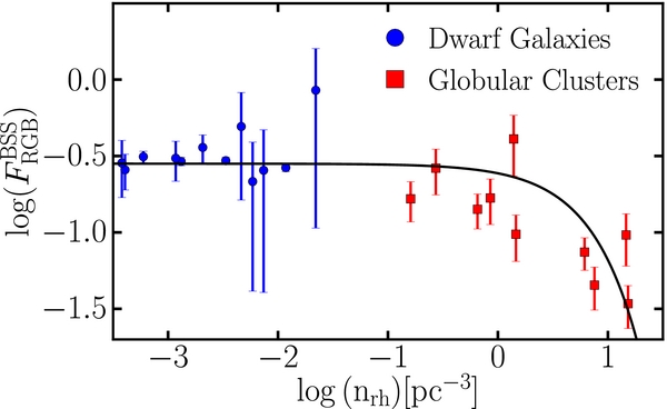
**Figure 6.** Specific fraction of blue stragglers $F_{\rm {RGB}}^{\rm {BSS}}$ plotted against density, calculated inside one half-light radius for each system. While dwarf galaxies show a flat distribution in the low-density regime, clusters show an anti-correlation in the high-density regime. The fitted function is shown as a solid black line, which corresponds to $\log ({F_{\rm {RGB}}^{\rm {BSS}}})$ ∝ (−0.063 ± 0.007) n_rh.
Download figure:
Standard image High-resolution image

**Figure 7.** Specific fraction of blue stragglers $F_{\rm {RGB}}^{\rm {BSS}}$ plotted against the rate of single–single star encounters, as calculated in Leigh & Sills (2011). The fitted function is $\log ({F_{\rm {RGB}}^{\rm {BSS}}})$ ∝ (−1.9 ± 0.2)× 10⁹ Γ and is illustrated as a solid black line.
Download figure:
Standard image High-resolution image

3.2. Blue Straggler/Young Star Discrimination

By definition, blue straggler stars live in a region of the CMD that could also be inhabited by young stars. In old systems without recent episodes of star formation, like the globular clusters have traditionally been considered, the identification of blue straggler stars in the CMD is straightforward. However, for satellites where recent episodes of star formation cannot be ruled out a priori, it is not immediately clear whether an observed extension of the MS beyond the older turnoff is due to blue stragglers or young stars.

We studied the numbers and magnitude distributions of stars inhabiting the region of the CMD occupied by blue stragglers. Based on these values, we estimate the ages and fractions of young stars that would reproduce our observations in the absence of genuine blue stragglers. In this way, we can assess the likelihood that recent bursts of star formation could be responsible for the stars observed beyond the MSTO.

Given the extremely low number of stars present in our dwarf galaxies, the only region of the CMD that we can use to compare blue stragglers and young stars is the region previously defined as our blue straggler box, since all the other regions of the CMD would show negligible numbers of blue stragglers and/or young stars compared to the main old population or contamination stars (see Figure 8 for an example of the expected appearance of a CMD where young stars could reproduce the number and distribution of stars observed beyond the MSTO in our dwarf galaxies).

**Figure 8.** Simulated CMD for fake stars with a young star fraction of 0.02. Red and blue points represent, respectively, 2 Gyr and 12 Gyr stars. The solid and dashed black lines show the theoretical isochrones used, while the blue and red boxes show the regions where blue straggler stars and RGB stars were counted, respectively.
Download figure:
Standard image High-resolution image

To estimate the properties of the young stars that could reproduce the blue straggler frequencies observed in our galaxies, we ran simulations where we generated both a young and an old single stellar population. To generate these populations, we used two Padova isochrones: a young one with an age varying from 1 to 3 Gyr and an old one with an age of 12 Gyr, both with an abundance of [Fe/H] =−2.0, which represents the average among the galaxy sample.⁸ We also used the corresponding theoretical luminosity functions, based on a Chabrier (2003) initial mass function, incorporating magnitude uncertainties consistent with our photometric data. Once we populated the fake CMDs, we counted blue straggler-like and RGB stars in the same way as we did for the real data. Thus, for a given age a and fraction of young stars f, we obtained a simulated blue straggler fraction F(a, f) corresponding to the one that a given system with no genuine blue stragglers would show. By comparing the frequencies measured in the real data and the simulated data, we obtained the fraction of young stars that would be needed to mimic the observed population of blue stragglers. In Figure 8, a simulated CMD is shown for illustration, with young and old populations of 2 and 12 Gyr, respectively, and a fractional number of young stars compared to total stars equal to 0.02. The results of the simulations are shown in Figure 9. This plot shows the fake blue straggler frequencies corresponding to different fractions of young stars, for ages ranging from 1 to 3 Gyr. Also shown here are the ranges of blue straggler fractions actually observed: one including all the objects and the other excluding the 4 (out of 12) galaxies with the largest frequency uncertainties.

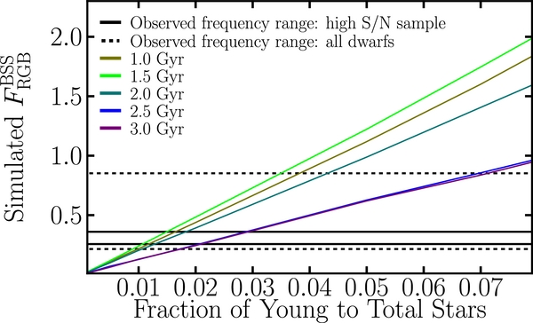
**Figure 9.** Simulated fraction of blue straggler stars corresponding to each young star fraction, for different ages of the generated stars. The black dashed lines show the blue straggler fraction range observed in our complete galaxy sample. The black solid lines show the blue straggler fraction range observed in the galaxies excluding the four systems with the highest frequency uncertainties.
Download figure:
Standard image High-resolution image

Additionally, we constrained the age of young stars that could mimic blue stragglers by comparing the magnitude distribution of each set of young stars with those of the observed blue stragglers. We also used the globular clusters as a "control sample." Given that the number of stars in the UFDs are extremely low, we analyzed the magnitude distribution of the UFDs as a single group in order to make the comparison statistically meaningful. The three classical dSphs in our sample were studied individually. We carried out a Kolmogorov–Smirnov (K-S) test to compare the different sets of stars and found that stars with ages of 2.5 ± 0.5 Gyr were the only ones even marginally consistent with the magnitude distribution of the observed blue stragglers in our dwarf galaxies. The magnitude distributions of blue stragglers in globular clusters are also consistent with the distribution of 2.5 Gyr old stars and blue stragglers from dwarf galaxies. This result comes as no surprise. For populations older than ∼2.5 Gyr, turnoff stars leave what we defined as our blue straggler box progressively closer to its faint end while younger populations will extend beyond the upper luminosity limit observed for blue stragglers, both in clusters and in galaxies.

What is left to determine is the fraction of stars with ages in the range of 2–3 Gyr that would reproduce the specific fractions of blue stragglers observed in our dwarf galaxies. Figure 9 shows that to reproduce the lowest observed fraction of blue straggler stars in all dwarf galaxies, a minimum young star fraction of ∼1%–2% is needed. For the upper limit, the fractions needed are ∼4%–7% for 2.5 ± 0.5 Gyr old stars.

In summary, the stars in the region of the CMD occupied by blue stragglers in our dwarf galaxies can be attributed to recent bursts of star formation only if all the dwarf galaxies in our sample formed stars 2.5 ± 0.5 Gyr ago and these stars account for ∼1%–7% of the total number of stars, or ∼1%–9% in mass fraction. Furthermore, if we exclude the four systems with the highest blue straggler frequency uncertainties, the fine-tuning of the star formation history of galaxies would have to be even greater to explain blue stragglers, since the young star fraction needed would have to be in the narrow range of 1% to 3%, which, as we explain in the discussion section, we deem highly unlikely.

3.3. Radial Distribution Analysis

We explored an additional line of evidence to help elucidate the nature of the blue straggler candidates in our Galactic satellites: we compared their radial distributions to those of RGB and MS stars. How blue stragglers are distributed throughout a system is the result of a complex interplay between dynamical history and the dominant blue straggler formation mechanism. In our dwarf galaxy sample, collisions are negligible and two-body relaxation times are longer than the age of the universe and therefore dynamical evolution (mass segregation) is not expected. In this scenario, there is no reason to presume a central concentration of blue stragglers. Young stars, on the other hand, tend to be centrally concentrated with respect to other stellar populations in dwarf galaxies (e.g., Harbeck et al. 2001; Grebel 2001), and thus the radial distribution of the stars we classified as blue stragglers can help us distinguish genuine blue stragglers from young stars. In the case of the globular clusters in our sample, where we can assume a priori that blue stragglers are genuine, eventual central concentration could shed some light on the relevance of collisions as a formation mechanism.

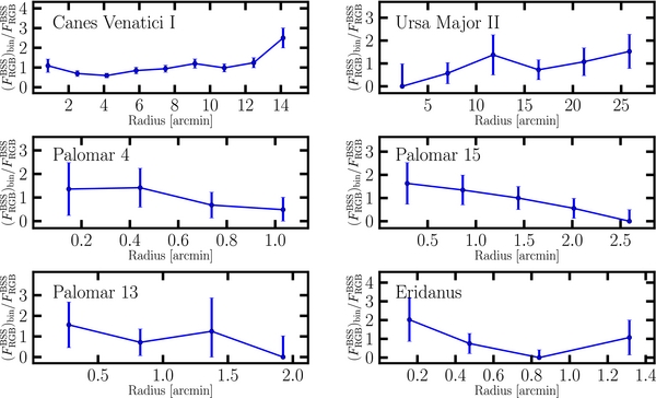
For most satellites in our sample, we found that the radial distribution of blue stragglers is nearly indistinguishable from that of RGB stars. Significant differences are seen only in 6/22 = 27% of our systems. These objects are: the UFDs Canes Venatici I and Ursa Major II and the globular clusters Palomar 4, Palomar 13, Palomar 15, and Eridanus. Figure 10 shows the blue straggler fraction versus radius, normalized by the overall fraction of blue stragglers, for these six objects. It is interesting that for Canes Venatici I and Ursa Major II, blue straggler stars are located preferentially in the outer regions. This behavior is also observed in galaxies like Draco, although for this galaxy the difference is too small for the K-S test to differentiate between both radial distributions. For the globular clusters in the figure, a clear radial concentration is observed (except for Eridanus, where a bimodal distribution might be present).

**Figure 10.** Radial distribution of blue stragglers with respect to the radial distribution of RGB stars. For each system, the curve shows the specific frequency of blue stragglers at different radii normalized to the total specific frequency of blue stragglers. All the objects where the radial distributions of blue stragglers were not statistically consistent with the radial distributions of RGB stars are plotted. Top: two dwarf galaxies where blue stragglers are located preferentially on the outskirts of the system. Middle: two globular clusters where blue stragglers are centrally concentrated. Bottom: globular cluster Palomar 13 (left panel) with a central concentration of blue stragglers and the Eridanus globular cluster (right panel), where a bimodal distribution may be present.
Download figure:
Standard image High-resolution image

It is worth reminding the reader that the area we used to select blue stragglers corresponds to twice the half-light radius of the systems, and therefore features in the radial distribution present at larger distances will not be observed if the objects extend much further than this. However, we do not anticipate this selection effect to be a problem given the extremely low densities at radii larger than 2 × r_h.

4. DISCUSSION

4.1. Dwarf Galaxies

In both classical and UFD galaxies, blue stragglers are ubiquitous, regardless of how low the stellar densities or encounter rates are. The specific frequencies of blue stragglers are high compared to those observed in globular clusters and are found to be statistically consistent with being constant over a 6 mag range. Given that we found the RGB populations to scale linearly with luminous mass, this result is equivalent to saying that the number of blue stragglers grows almost linearly with the total stellar mass of the system.

We used simulations of young populations to compare their photometric properties with those of the blue stragglers observed in dwarf galaxies and conclude that the latter are genuine, as opposed to young stars. A number of facts support this conclusion: (1) for young stars to have magnitude distributions statistically consistent with those of the blue stragglers observed in dwarf galaxies, their ages need to be closely clumped around 2.5 Gyr. This result can be readily understood when we consider that our brightest blue stragglers have an absolute magnitude of M_g ∼ 1.9, coincident with the magnitude at which a 2.5 Gyr old star evolves out of our blue straggler star box. This is also the magnitude corresponding to a star with twice the mass of a turnoff star 12 to 13 Gyr old, an expected result if we are seeing blue stragglers formed by collisions (either single–single or in binaries) or mass-transfer in binary systems. (2) The magnitude distributions of blue stragglers in both dwarf galaxies and globular clusters (where they can be reliably classified as blue stragglers) are completely consistent. (3) The lack of central concentration of blue stragglers in dwarf galaxies is consistent with the scenario wherein these stars form from mass-transfer or mergers in primordial binaries or multiple systems, rather than being the result of a recent star formation episode. In the latter case, the young stars would be expected to be located preferentially near the central regions. (4) From the simulations, we also determined that the 2.5 ± 0.5 Gyr old stars should constitute 1%–7% of the total number of stars in all the dwarf galaxies in our sample in order to reproduce the range of observed blue straggler frequencies. This result implies an unlikely fine-tuned star formation history.

Most galaxies in our sample have half-light densities of 10⁻²–10⁻³ stars pc⁻³, i.e., at least 10 times less dense than the solar neighborhood (Latyshev 1978). Given these extremely low stellar densities, blue stragglers formed by collisions between stars can be safely ruled out. When considering collisions between single, binaries, or triple stars, the collision times (calculated as in Leigh & Sills 2011) are orders of magnitude larger than the age of the universe. Even though some physical processes have been particularly successful in explaining collisions in low-density environments, they might not explain the blue stragglers observed in systems like our dwarf galaxies. For instance, the triple evolution dynamical instability proposed by Perets & Kratter (2012) produces encounter rates that are too low in systems with low numbers of stars to explain our dwarf galaxy blue stragglers.

If collisions of any kind cannot account for blue stragglers in our systems, their presence can only be explained if they formed via mass-transfer and/or mergers in primordial binaries, whether or not they have more companion stars that are members of the system. Two powerful correlations were found to support this claim. When plotting blue straggler fractions against both density and encounter rate, we found that a single exponential function could reproduce the behavior of all satellites in our sample. In this context, dwarf galaxies live in the lower density/encounter rate regime, displaying high and similar values of blue straggler fractions. These results point to the fact that collisions neither significantly create nor prevent the formation of blue stragglers. On the other hand, as we explain below, close encounters in higher density environments prevent blue straggler formation by altering the configuration of the binary or multiple systems. Finally, the lack of central concentration of blue stragglers in all our dwarf galaxies is also consistent with the binary/multiple system scenario, implying that these stars can be formed in all regions of our galaxies and not just their slightly higher density central regions.

The similarity in the blue straggler fractions observed in galaxies can be explained if the primordial binary star fractions are also similar. While this should be further confirmed by observations, hints that this is in fact the case already exist; Geha et al. (2013) measured the binary fraction of two ultra-faint galaxies and found an identical binary fraction of 47%.

4.2. Globular Clusters

Our observations show that, for the globular clusters in our survey, the specific frequency of blue stragglers decreases when there is an increase in a particular physical parameter of the host system, such as luminosity, stellar densities, encounter rate, and total stellar mass. The anti-correlation between $F^{\rm {BSS}}_{\rm {RGB}}$ and the luminosity of the systems is similar to the one observed for inner halo clusters, even though our globular clusters are on average less luminous and larger (5–10 ×). The slope of our anti-correlation is consistent within the uncertainties with the one found by Piotto et al. (2004) using a sample of 56 globular clusters with −6 > M_V > −10, and by Sandquist (2005), who extended the results of Piotto et al. with lower luminosity clusters down to M_V ∼ −4. The anti-correlation derived in our study extends the existing ones to absolute magnitudes as faint as M_V ∼ −2.5. At this faint end, the fraction of blue straggler stars in our globular clusters is comparable to that of dwarf galaxies. Despite the consistency between our correlations, there is a key difference between our results and the ones of Piotto et al. (2004): we study blue stragglers within 2 × r_h of our clusters, which represents a significant fraction of the total cluster area, whereas Piotto's work focused on the cluster cores. This difference is important since, as proposed by Leigh et al. (2011a), the systems with the longer relaxation times/higher mass would not have had time to sink their blue stragglers to the innermost regions by two-body relaxation. This would reduce the number of blue stragglers, N_BSS, found in the high-mass clusters when counting them in the most central regions, but that would not affect the trend of N_BSS when the region of the cluster considered represents a considerable fraction of the total cluster area. Thus, if dynamics in the central regions do not destroy the progenitors of blue stragglers and these stars are homogeneously formed within the clusters, mass segregation would translate to a sublinear dependence of N_BSS with cluster mass enclosed when studying only the central regions, whereas a linear dependence would be expected when considering larger areas. Our Figure 5 then argues against mass segregation playing an important role in the blue straggler counts in our globulars.

As was the case for dwarf galaxies, collisions alone are unable to explain the fraction of blue stragglers observed in our globular clusters. Based on the collision times, calculated as in Leigh & Sills (2011), collisions between single, binary, or triple systems can account only for a small contribution to the blue straggler numbers observed in our highest density clusters. Thus, there should be another dominant blue straggler formation mechanism at work. Figures 6 and 7 show that globular clusters inhabit our higher density, higher encounter rate regime; these objects show a systematic decrease in blue straggler fraction with both physical parameters. We interpret these trends as supporting a scenario where mass-transfer or mergers in binary or multiple star systems are the dominant blue straggler formation mechanism in the outer halo globular clusters. The following pieces of evidence support this scenario: (1) the behavior of the frequency of blue stragglers is well fit by single trends with smooth transitions between dwarf galaxies and clusters, which points to a common origin for their blue stragglers. (2) A systematic decrease of the blue straggler fraction with encounter rate and density is inconsistent with the collision scenario. Instead, this result points to encounters preventing blue straggler formation in our globular clusters. (3) The expressions shown in Equations (6) and (7) describing the exponential decay of the frequency of blue stragglers with both density and encounter rate arise naturally if the relative decrease in the fraction of blue stragglers varies as the ratio between the age of the system and the collision time. It is worth pointing out that collisional blue stragglers might have shorter lifetimes than systems formed through mass transfer (Chatterjee et al. 2013). This means that we cannot rule out the possibility that a fraction of blue stragglers in denser systems still formed through collisions involving binaries (that would have otherwise undergone mass transfer to form a blue straggler) and that they quickly evolved away from the blue straggler region. We argue that this would be only a second order effect, because the differences in the lifetimes of blue stragglers produced by the different mechanisms is much less than the differences needed to explain the decline in the frequency of blue stragglers observed for our clusters.

Aside from our study, there is mounting evidence favoring a binary origin for blue stragglers. A direct link between blue straggler stars and binaries has been determined by Preston & Sneden (2000), who derived a binary fraction of 68% among their metal-poor field blue straggler stars, and Mathieu & Geller (2009), who estimated a binary fraction of 76% among blue straggler stars in NGC 188. Palomar 13, one of the clusters with the highest blue straggler frequencies, is known to have a relatively high fraction of binary stars, 30% ± 4% (Clark et al. 2004), and many of this cluster's blue straggler stars were shown to exhibit significant velocity variations, suggesting that these objects are unresolved binary systems (Bradford et al. 2011).

In our globular cluster sample, the radial distributions of blue stragglers are in most cases indistinguishable from those of RGB or MS stars, consistent in principle with the binary scenario. However, a clear central concentration of blue stragglers is observed in a few clusters: Palomar 4, Palomar 13, and Palomar 15, while a bimodal distribution might be present in Eridanus. At first glance, this result may seem contradictory with our interpretation of Figure 6 that higher density environments favor the destruction or separation of binary or multiple system progenitors of blue stragglers, but the trend of frequency with density followed by different objects should not necessarily be expected to hold within a single system. Fregeau et al. (2009) studied the evolution of binaries in dense stellar systems and found an increase with time of the core binary fraction, which could be understood as a consequence of a complex interaction between the mass segregation of binaries in the core and their subsequent destruction there. In addition, once formed, blue stragglers can also migrate toward the central regions through mass segregation. In summary, dynamical processes likely to occur in globular clusters severely complicate the interpretation of the trends observed within an individual object.

5. CONCLUSIONS

We have presented a comprehensive analysis of the blue straggler star population in a representative subsample of Galactic outer halo satellites. This photometrically homogeneous sample includes ten low-density globular clusters, three classical dSph galaxies, and nine of the recently discovered UFD galaxies. Despite their diverse physical properties, all these satellites are relatively loose and scarcely populated when compared to inner halo globular clusters, where most blue straggler star studies have been carried out. Given the extremely long collision times of our systems, collisions involving single, binary, or triple stars can only account for a small fraction of the blue stragglers of our highest density clusters, while their influence on dwarf galaxies should be negligible. Our sample provided an opportunity to study blue straggler populations in a new density/luminosity regime. We claim that the dominant blue straggler formation mechanism in these type of systems is mass-transfer or mergers in binary or multiple star systems. In the higher encounter rate regime spanned by our globular clusters, encounters prevent blue straggler formation by altering the configuration of the star systems that would otherwise produce blue straggler stars.

Our results can be summarized as follows.

1.
We found blue stragglers to be ubiquitous among globular clusters and dwarf galaxies, including the UFDs.
2.
The blue straggler populations in both classical dSphs and UFDs show a remarkably high and constant distribution of their fractions over an absolute magnitude range of more than 6 mag, and a density range of two orders of magnitude.
3.
The behavior of the frequency of blue stragglers is well fit by single trends with smooth transitions between dwarf galaxies and clusters, which points to a common origin for their blue stragglers.
4.
The fraction of blue straggler stars is high and flat in the extremely low encounter rate regime spanned by dwarf galaxies, while it decreases exponentially with increasing stellar density or encounter rate for the regime spanned by our outer halo globular clusters.
5.
There is a well-defined anti-correlation between the fraction of blue straggler stars and absolute magnitude for the outer halo clusters in our sample. This trend has already been observed in inner halo clusters and it is also interpreted as a consequence of the binary origin of the blue straggler population.
6.
Comparing the magnitude distribution of the observed blue stragglers in dwarf galaxies with those of simulated single stellar populations, we find that for blue stragglers in dwarf galaxies to be young stars, they would have to correspond to a 2.5 ± 0.5 Gyr old population. In addition, to match the observed blue straggler fractions seen in galaxies, young stars would have to comprise between ∼1%–7% of the total number of stars. Such fine-tuned requirements make it unlikely that we are mistakenly classifying young stars as blue stragglers.
7.
The radial distribution of blue stragglers in most objects is statistically consistent with the radial distributions of RGB and MS stars. Only a few exceptions are found, notably the central concentration seen in Palomar 4, Palomar 13, Palomar 14, and the bimodal distribution in Eridanus. In all these cases, dynamical processes, such as mass segregation, are likely to alter the primordial binary population and therefore the interpretation of the trends observed within individual objects is not straightforward.

We thank the referee for very useful comments that helped improve this paper significantly. F.A.S. thanks Andrés Guzmán for useful discussions. F.A.S. acknowledges support from CONICYT-PCHA/Doctorado Nacional/2010-21100133. R.R.M. acknowledges partial support from CONICYT Anillo project ACT-1122 and project BASAL PFB-06 as well as from the FONDECYT project N°1120013. M.G. acknowledges support from the National Science Foundation under award number AST-0908752 and the Alfred P. Sloan Foundation. S.G.D. was supported in part by the NSF grant AST-0909182 and by the Ajax Foundation. This work was supported in part by the facilities and staff of the Yale University Faculty of Arts and Sciences High Performance Computing Center.

A MEGACAM SURVEY OF OUTER HALO SATELLITES. II. BLUE STRAGGLERS IN THE LOWEST STELLAR DENSITY SYSTEMS^*

Article metrics

Permissions

Author e-mails

Author affiliations

Dates

ABSTRACT

1. INTRODUCTION

2. DATA AND BLUE STRAGGLER SELECTION