


ABSTRACT
We present measurements of the auto- and cross-frequency power spectra of the cosmic infrared background (CIB) at 250, 350, and 500 μm (1200, 860, and 600 GHz) from observations totaling ∼70 deg2 made with the SPIRE instrument aboard the Herschel Space Observatory. We measure a fractional anisotropy δI/I = 14% ± 4%, detecting signatures arising from the clustering of dusty star-forming galaxies in both the linear (2-halo) and nonlinear (1-halo) regimes; and that the transition from the 2- to 1-halo terms, below which power originates predominantly from multiple galaxies within dark matter halos, occurs at kθ ∼ 0.10–0.12 arcmin−1 (ℓ ∼ 2160–2380), from 250 to 500 μm. New to this paper is clear evidence of a dependence of the Poisson and 1-halo power on the flux-cut level of masked sources—suggesting that some fraction of the more luminous sources occupy more massive halos as satellites, or are possibly close pairs. We measure the cross-correlation power spectra between bands, finding that bands which are farthest apart are the least correlated, as well as hints of a reduction in the correlation between bands when resolved sources are more aggressively masked. In the second part of the paper, we attempt to interpret the measurements in the framework of the halo model. With the aim of fitting simultaneously with one model the power spectra, number counts, and absolute CIB level in all bands, we find that this is achievable by invoking a luminosity–mass relationship, such that the luminosity-to-mass ratio peaks at a particular halo mass scale and declines toward lower and higher mass halos. Our best-fit model finds that the halo mass which is most efficient at hosting star formation in the redshift range of peak star-forming activity, z ∼ 1–3, is log(Mpeak/M☉) ∼ 12.1 ± 0.5, and that the minimum halo mass to host infrared galaxies is log(Mmin/M☉) ∼ 10.1 ± 0.6.
Export citation and abstract BibTeX RIS
1. INTRODUCTION
Star formation is well traced by dust, which absorbs the UV/optical light produced by young stars in actively star-forming regions and re-emits the energy in the far-infrared/submillimeter (FIR/submm; e.g., Savage & Mathis 1979). Roughly half of all starlight ever produced has been reprocessed by dusty star-forming galaxies (DSFGs; e.g., Hauser & Dwek 2001; Dole et al. 2006), and this emission is responsible for the ubiquitous cosmic infrared background (CIB; Puget et al. 1996; Fixsen et al. 1998). The mechanisms responsible for the presence or absence of star formation are partially dependent on the local environment (e.g., major mergers: Narayanan et al. 2010; condensation or cold accretion: Dekel et al. 2009, photoionization heating, supernovae, active galactic nuclei, and virial shocks: Birnboim & Dekel 2003; Granato et al. 2004; Bower et al. 2006). Thus, the specifics of the galaxy distribution—which can be determined statistically to high precision by measuring their clustering properties—inform the relationship of star formation and dark matter density, and are valuable inputs for models of galaxy formation. However, measuring the clustering of DSFGs has historically proven difficult to do.
Owing to the relatively large point-spread functions (PSFs) of ground-, balloon-, and space-based submillimeter observatories, coupled with very steep source counts, maps at these wavelengths are dominated by confusion noise. For the 250 μm channel on Herschel, for example, this means that no matter how deeply you observe a field, without some sort of spatial deconvolution at best only ∼15% of the flux density will be resolved into individually detected galaxies (Oliver et al. 2010b). Adding to that the fact that the redshift distribution of DSFGs is relatively broad (e.g., Casey et al. 2012; Chapman et al. 2005; Béthermin et al. 2012c), clustering measurements of resolved sources have consequently had limited success (e.g., Blain et al. 2004; Scott et al. 2006; Weiß et al. 2009) and somewhat contradictory results (e.g., Cooray et al. 2010; Maddox et al. 2010).
The remaining intensities in the maps appear as fluctuations, or anisotropies, in the CIB. Contained in CIB anisotropies (or CIBA) is the clustering pattern, integrated over luminosity and redshift, of all DSFGs—including those too faint to be resolved. And analogous to the two-point function typically used to estimate the clustering of resolved galaxies, the power spectrum of these intensity fluctuations is a probe of the clustering properties of those galaxies (e.g., Bond & Efstathiou 1984; Scott & White 1999; Knox et al. 2001; Negrello et al. 2007). Initial power spectrum measurements from Spitzer (Grossan & Smoot 2007; Lagache et al. 2007), BLAST (Viero et al. 2009; Hajian et al. 2012), ACT (Dunkley et al. 2011), and SPT (Hall et al. 2010) found a signal in excess of Poisson noise originating from the clustering of DSFGs, but were limited to measuring the galaxy bias in the linear regime, rather than their distribution within dark matter halos. Subsequent measurements from Herschel/SPIRE (Amblard et al. 2011) and Planck (Planck Collaboration et al. 2011b) were able to isolate the linear and nonlinear clustering signals, but the two groups found that their measurements agreed only after correcting for multiple systematics.
Power spectra can be interpreted with modeling frameworks in much the same way as is done for two-point function measurements of resolved sources. Among the most commonly adopted models are so-called halo models (e.g., Seljak 2000; Cooray & Sheth 2002), which use halo occupation distributions (e.g., Peacock & Smith 2000; Scoccimarro et al. 2001) to statistically assign galaxies to dark matter halos in order to recreate observed clustering measurements. Halo models have been adopted to interpret CIBA spectra from BLAST (Viero et al. 2009), Herschel/SPIRE (Amblard et al. 2011; Pénin et al. 2012a; Xia et al. 2012), and Planck (Planck Collaboration et al. 2011b; Pénin et al. 2012a; Shang et al. 2012; Xia et al. 2012), with varying success.
Precisely measuring the CIBA power spectra and decoding the information contained within them is a rapidly growing field, and it is also the focus of this paper. First and foremost, we aim to advance the field by providing state-of-the-art measurements of the auto- and cross-frequency power spectra of CIBA at 250, 350, and 500 μm, spanning angular scales 0.01 ⩽ kθ ≲ 2 arcmin−1 (or 350 ≲ ℓ ≲ 45, 000) (Section 4). With the addition of more than four times the area, we extend the efforts of Amblard et al. (2011)—who definitively resolved a signature of nonlinear clustering on small scales—by illustrating how the strength of the nonlinear clustering signal depends strongly on the flux-cut level of masked sources (Section 4.4.1). We improve on the efforts of BLAST (Viero et al. 2009; Hajian et al. 2012) by measuring the cross-frequency power spectra and estimate the level of correlation between bands (Section 4.5).
We then attempt to interpret our measurements with a series of halo models, whose common feature is to tie the luminosities of sources to their host halo masses (Section 5.1), but which differ by their treatment of the spectral energy distribution (SED) of galaxy emission. Our models fit the auto- and cross-frequency power spectra in each band and measured number counts of sources, simultaneously, thereby introducing a new level of sophistication to the body of existing halo models in the literature. When required, we adopt the concordance model, a flat ΛCDM cosmology with ΩM = 0.274, ΩΛ = 0.726, H0 = 70.5 km s−1 Mpc−1, and σ8 = 0.81 (Komatsu et al. 2011).
2. DATA
The primary data set for this work comes from the Herschel Multi-tiered Extragalactic Survey34 (HerMES; Oliver et al. 2012), a guaranteed time key project of the Herschel Space Observatory (Pilbratt et al. 2010). We use submillimeter maps observed with the SPIRE instrument (Griffin et al. 2010) at 250, 350, and 500 μm. We also use reprocessed 100 μm IRAS (Neugebauer et al. 1984) maps in order to quantify the contribution to the power spectra from Galactic cirrus (see Section 3.3). Each of the data sets is described in detail below.
2.1. HerMES/SPIRE
HerMES fields are organized, according to area and depth, into levels 1 through 7, with Level 1 maps being the smallest and deepest (∼310 arcmin2), and level 7 maps the widest and shallowest (∼270 deg2; Oliver et al. 2012).
This study focuses on a subset of the level 5 and 6 fields, totaling ∼70 deg2, chosen for their large area and uniformity, and because they have a manageable level of Galactic cirrus contamination. The fields used for this study, and a summary of their properties, are given in Table 1. Combined, they represent an increase of more than four times the area of the initial HerMES study (Amblard et al. 2011). The largest of the HerMES fields, the HerMES Large-Mode Survey (HeLMS)—which was designed specifically to measure the power spectrum on large angular scales—is still in preparation, and will be the subject of a future study. Maps will be made available to the public through HeDaM35 (Roehlly et al. 2011) as a part of data release 2.
Table 1. Map Properties of the HerMES Fields
| Field Name | Area | 1σ Noise | Repeats | Scan Speed |
|---|---|---|---|---|
| (deg2) | (MJy sr−1) | No. | ||
| bootes | 11.3 | 1.11, 0.61, 0.29 | 9 | Parallel |
| cdfs-swire | 12.2 | 1.00, 0.57, 0.27 | 5/20 | Parallel/Fast |
| elais-s1 | 8.6 | 1.12, 0.63, 0.31 | 8 | Parallel |
| lockman-swire | 15.2 | 1.08, 0.60, 0.29 | 4/20 | Parallel/Fast |
| xmm-lss | 21.6 | 1.15, 0.68, 0.52 | 8 | Parallel |
Notes. Total noise (1σ including confusion) is given at 250, 350, and 500 μm, respectively. Repeats are defined as the number of times a field has been observed in two orthogonal passes, thus one repeat equals two passes. cdfs-swire and lockman-swire were observed partially in Parallel mode, and partly in Fast mode. The scan speed of the telescope is either 20 arcsec s−1 (Parallel) or 60 arcsec s−1 (Fast).
Download table as: ASCIITypeset image
The data obtained from the Herschel Science Archive were processed with a combination of standard ESA software and a customized software package SMAP. The maps themselves were then made using an updated version of SMAP/SHIM (Levenson et al. 2010), an iterative map-maker designed to optimally separate large-scale noise from signal. SMAP differs from HIPE (Ott 2010) in three fundamental ways which are relevant for power spectrum studies. First, the standard scan-by-scan temperature drift correction module within HIPE is overridden in favor of a custom correction algorithm which stitches together all of the time-ordered data (or timestreams), allowing us to fit to and remove a much longer noise mode. Further, the standard processing is modified such that a "sigma-kappa" deglitcher is used instead of a wavelet deglitcher, to improve performance in large blank fields. Lastly, imperfections from thermistor jumps, the "cooler burp" effect, and residual glitches are removed manually before map construction. Detailed descriptions of the updates to the SMAP pipeline of Levenson et al. (2010) are presented in Appendix A.
Following Amblard et al. (2011), we make maps with 10 iterations, fewer than SMAP's default of 20, in order to minimize the time needed to measure the transfer functions (Section 3.1.2) and uncertainties (Section 3.2) with Monte Carlo simulations.
Additionally, timestream data are divided into two halves and unique "jack-knife" map-pairs are made. These map-pairs are those ultimately used for estimating power spectra (Section 3.1). SMAP maps are natively made with pixel sizes of 6'', 8 33, and 12'', which is motivated by the beam size (sampling them by ∼1/3 FWHM). But because the cross-frequency power spectra calculations need maps of equivalent pixel sizes, three additional sets of map-pairs are made, with the extra sets having custom pixel sizes so that the cross-frequency power spectra can be performed at the pixel resolution native to the maps with the larger instrumental beams. In other words, the maps used to calculate the 250 × 350 μm spectra have identical 833 pixels, and those used for 250 × 500 and 350 × 500 μm have 12'' pixels.
2.2. IRAS/IRIS
At 100 μm, we use the Improved Reprocessing of the IRAS Survey36 (IRIS; Miville-Deschênes & Lagache 2005), a data set which corrects the original plates for calibration, zero level, and striping problems. The resulting FWHM resolution and noise level are 4 3 ± 02 and 0.06 ± 0.02 MJy sr−1, respectively, and the gain uncertainty is 13.5%. Data are available for up to three independent observations, or HCONs, although two of our fields were only observed twice. For fields in which tiles intersect, maps can be stitched together with custom software provided on their site.37
3. POWER SPECTRUM OF CIB ANISOTROPIES
The CIB at submillimeter wavelengths is dominated by emission from DSFGs, while other potential sources of signal, like the cosmic microwave background (CMB), Sunyaev–Zel'dovich effect, GHz-peaking radio galaxies or quasars, and intergalactic dust, are subdominant and can be safely ignored. Anisotropies arise from galaxy overdensities (i.e., galaxy clustering) which appear as background fluctuations. These anisotropies can be described by their power spectrum, and are made up of the following contributions:

Here  is Poisson (or shot) noise,
  is the power resulting from the clustering of galaxies, i.e., the excess above Poisson,
  is the noise from foregrounds, and Ninst is the instrumental noise. The foreground noise term could in principle include Galactic cirrus, free-free, synchrotron, and zodiacal emission, but in practice all but the cirrus term are negligible at SPIRE's wavelengths (e.g., Hajian et al. 2012).
The Poisson noise component arises from the discrete sampling of the background, and as such is decoupled from the clustering term. For sources with a distribution of flux densities dN/dSν the effective Poisson level is
while the clustered power for the same sources can be estimated as roughly the three-dimensional power spectrum of the galaxy number density field weighted by the square of the redshift distribution of the cumulative flux, (dSν/dz)2.
The contribution to the Poisson noise and clustered power from galaxies with different flux densities are illustrated as solid and dashed lines in Figure 1, respectively. The peak contribution to the Poisson noise is from galaxies with Sν ≈ 22, 14, and 8 mJy at 250, 350, and 500 μm, while the peak contribution to the clustering power comes from fainter (higher-z) sources, with S ≈ 7, 5, and 3 mJy at 250, 350, and 500 μm. Shown as dotted vertical lines at ∼90, 75, and 60 mJy are the 5σ limits of resolved sources in maps of equivalent depth (Nguyen et al. 2010). Poisson noise in the power spectrum is flat (in units of Jy2 sr−1), behaving as a level of white noise which can be reduced by masking brighter sources. Note that masking sources is more effective at reducing the Poisson level at 250 μm than it is at 350 or 500 μm.

Figure 1. Differential (top panel) and cumulative (bottom panel) contributions to the Poisson (solid lines) and clustering (dashed lines) power from sources of different flux densities, estimated from the Béthermin et al. (2011) model for illustrative purposes. Top panel: the Poisson curves are determined by the normalization of S3dN/dS and the clustering curves of S4(dN/dS)2. By multiplying by an additional power of S, the peak values represent where the contribution to the integral per logarithmic interval is maximum. The integral under the curves for Scut < 73, 61, and 88 mJy at 250, 350, and 500 μm, respectively (dotted vertical lines)—which represent the 5σ source detection threshold for a map made with five repeats—are set equal to unity. The median values of sub-100 mJy local maxima are (Poisson) 22, 14, and 8 mJy, and (CIB) 7, 5, and 3 mJy, at 250, 350, and 500 μm, respectively. Bottom panel: cumulative contribution to the power spectra normalized to unity at the detection threshold. It is evident from this that the Poisson level at 250 μm, and to a lesser extent at 350 μm, is very sensitive to the masking level of resolved sources, while the 500 μm channel is fairly insensitive to source masking. The clustering signal, on the other hand, is largely insensitive to masking. Note that the clustering curves are estimates of linear clustering power, and do not include nonlinear effects which may be more sensitive to source masking.
Download figure:
Standard image High-resolution image3.1. Estimating the Power Spectra: Masking, Filtering, and Transfer Functions
The intensity in a given SPIRE map, Imap, can be approximated as

where Isky is the sky signal we wish to recover, T is the transfer function of the map-maker, B is the instrumental beam, N is the noise, and W is the window function, which includes the masking of map edges and of bright sources. We use ⊗ to represent a convolution in real-space. The instrumental noise, N, is made up of white noise, which dominates on angular scales kθ ≳ 0.2 arcmin−1, and 1/f noise. We note that as T has structure in 2D, and as the true beam may vary slightly across the map (particularly for bigger maps). These corrections are small enough that Equation (3) remains a reasonable approximation.
In the auto-correlation of a map (i.e., the auto-power spectrum of a single map), all of the power present—which includes both signal and noise—is correlated, while in the cross-correlation of jack-knife map-pairs, in principle the only signal correlated between them is the sky signal. Since we are interested in recovering the sky signal, we estimate the power spectrum from the cross-correlation of jack-knife map-pairs (discussed in Section 2.1). In practice, some correlated noise could exist between maps, particularly on large scales, as 1/f. To minimize this, we use map-pairs constructed by dividing the timestreams in half by time, which ensures that the maps are made from data taken at time intervals corresponding to very large scales. Note, this would not be true if, say, the data were split into those from even and odd detectors, since the same large-scale noise would be present in both maps. The remaining 1/f results from serendipitous alignment of large-scale noise (see Appendix B of Hajian et al. 2012), i.e., independent noise clumps in either map that happen to line up. Also note that excessive high-pass filtering of the time-ordered data before constructing maps would attenuate extragalactic large-scale signal along with unwanted signal, and is thus not employed.
The one-dimensional power spectrum is the azimuthal average of the (nearly isotropic) two-dimensional power spectrum of map-pairs in k-space. In order to recover the true power spectrum of the sky, the cross-spectrum of the map-pairs must be corrected for the transfer function, masking, and instrumental beam. We now describe these corrections in detail.
3.1.1. Masking and the Mode-coupling Matrix
Before calculating the power spectra, the maps are multiplied with windows whose values equal unity in the clean parts of the maps and taper to zero with a Gaussian profile (90'' FWHM) at the edges. Note that jack-knife maps typically do not cover identical patches of sky because the orientation of the telescope between observations changes, so that the windows of the two jack-knife map-pairs are different.
Next, because we are interested in the behavior of the power spectrum with the masking level of resolved point sources, we create a series of masks for each field and band to mask sources whose flux densities are greater than 50, 100, 200, and 300 mJy, in addition to extended sources. Extended sources are exceptional objects, e.g., local IRAS galaxies, which exceed 400 mJy but can be as bright as 1500 mJy at 250 μm. Mask positions are determined from catalogs of resolved sources which we construct. The source identification code first high-pass filters the maps in Fourier space to remove Galactic cirrus and other large-scale power, then convolves the maps by the instrumental beam, and finally measures all peaks with signal-to-noise ratio greater than 3σ. The total number of masked sources in each field and band is tabulated in Table 2. Note that this method could potentially suffer from Eddington bias (e.g., Chapin et al. 2009), a phenomenon where instrumental white noise systematically boosts faint sources above the detection limit. To ensure that this is not a significant problem, we compare the total number of sources above the cut to cumulative number counts from Glenn et al. (2010) and find that they are consistent.
Table 2. Number of Masked Sources
| ObsID | 300 mJy | 200 mJy | 100 mJy | 50 mJy |
|---|---|---|---|---|
| 18 | 38 | 180 | 1567 | |
| bootes | 4 | 9 | 46 | 723 |
| 1 | 2 | 13 | 248 | |
| 9 | 23 | 165 | 1569 | |
| cdfs-swire | 3 | 6 | 30 | 725 |
| 1 | 1 | 6 | 141 | |
| 9 | 23 | 104 | 1073 | |
| elais-s1 | 1 | 3 | 22 | 437 |
| 1 | 1 | 3 | 146 | |
| 16 | 42 | 221 | 2043 | |
| lockman-swire | 4 | 9 | 57 | 930 |
| 1 | 3 | 10 | 220 | |
| 23 | 66 | 368 | 2973 | |
| xmm-lss | 5 | 13 | 85 | 1170 |
| 1 | 2 | 16 | 437 | |
Notes. Number of sources masked at 250, 350, and 500 μm is given from top to bottom in each panel. Not accounted for in the table are the extended sources masked in each field, of which there are 3, 2, 2, 4, and 4, respectively. A 50 mJy cut amounts to masking approximately 1.4%, 1.2%, and 0.5% of the pixels at 250, 350, and 500 μm, respectively.
Download table as: ASCIITypeset image
Each source is masked by circles of 1.1 × FWHM in diameter, or 191, 277, and 403 at 250, 350, and 500 μm, respectively—chosen to cover the full first lobe of the beam, though we check that the exact size of the mask has a negligible effect on the spectra. For the data that concern this paper, unique masks are made for each field and each band (i.e., one at 250, one at 350, and one at 500 μm), so that only sources above the given cut in that band are masked. This means that when calculating the cross-frequency power spectra, not all of the sources masked at, e.g., 250 μm will also be masked at 350 μm, and vice versa. However, we additionally calculate an alternative set of spectra where we mask in all bands the sources identified at 250 μm (i.e., the same mask at 250, 350, and 500 μm), and the power spectrum pipeline is rerun. Plots and tables for this alternate masking scheme are presented in Appendix D, where we also show that the spectra at longer wavelengths are less sensitive to the level of source masking than at shorter wavelengths. Finally, we note that this method differs from that of Amblard et al. (2011), who instead masked all pixels above 50 mJy, as well as all neighboring pixels, the motivation being that a catalog-based masking scheme is better able to distinguish sources from spurious noise. The total number of masked sources in each field and band is tabulated in Table 2.
Masking in map-space can result in mode-coupling in Fourier space, which can bias the power spectrum. The coupling kernel, or mode-coupling matrix (Hivon et al. 2002), in the flat sky approximation is
where  is the auto-power spectrum of the mask, and N(θk) is the number of modes in annulus of radius k. Since in our case the masks of the map-pairs are not identical, Equation (4) is generalized for different masks by replacing
  with the cross-power spectrum of the masks,
  (see Tristram et al. 2005).
The mode-coupling matrix must be inverted in the final step in order to recover the de-coupled power spectrum. A unique mode-coupling matrix is calculated for each auto- and cross-frequency power spectrum, and for each flux cut, per field. Additionally, each  is tested on 1000 simulated maps with steep input spectra and found to be unbiased.
3.1.2. Transfer Function
The large-scale correlated noise of SPIRE is extremely low (e.g., Pascale et al. 2011). As a result, only minimal high-pass filtering is required to make well-behaved maps, and the resulting power spectrum can be measured out to relatively large scales (kθ ≳ 0.01 arcmin−1). This filtering is quantified by the transfer function of the map-maker, T, which must be accounted for in the final spectra.
We measure T with a Monte Carlo simulation whose steps are: (1) running the SMAP map-making pipeline on simulated observations of input maps with known power spectra resembling those of clustered DSFGs; (2) calculating the power spectrum of the output map with a pipeline identical to that used for the real data, including all masking, Fourier space filtering, and mode-coupling corrections; and (3) computing the average of the ratio of the output power spectrum to the known input spectrum. Transfer functions are calculated from 100 simulations of each field and wavelength, and are shown in Figure 2. We check that the spectra in step (1) are not sensitive to the steepness of the input spectra, and that the transfer functions have converged, with a mean error of ∼1%.
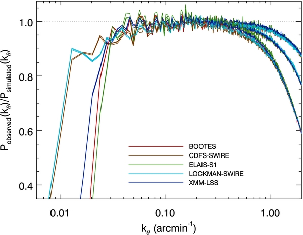
Figure 2. Transfer functions of the map-maker, averaged in 2D, for each of our fields. For any given field, the transfer functions on large scales are indistinguishable between bands, while on small scales, the transfer functions converge to that of the pixel windows, which are band dependent. The shape of the transfer function depends largely on: the scan speed, which determines on what scales the 1/f noise is projected onto the timestreams; and scan lengths, which determine the order of polynomial which is removed from the timestreams in the SMAP pipeline. Thus, maps which are smaller or which were observed with slower scans are attenuated on smaller angular scales.
Download figure:
Standard image High-resolution imageAs anticipated, all three bands converge on large scales for each field, meaning that the same filtering is performed in each band. And on small scales (kθ > 0.3 arcmin−1) all fields converge to the same three curves, which are the pixel window functions of the three bands. The angular scales on which the high-pass filtering occurs in each field are related to the average speeds and lengths of the maps scans: the former determines the scale in which 1/f noise is projected onto the timestreams, while the latter dictates the order of the polynomial removed from the timestreams. As described later in Section 4.2, the final spectra are weighted combinations of those in each field which are attenuated by less than 50%, corresponding to kθ ⩾ 0.021, 0.009, 0.023, 0.015, and 0.009 arcmin−1, for bootes, cdfs-swire, elais-s1, lockman-swire, and xmm-lss, respectively. Maps scanned with longer and faster scans have less attenuation on large scales, which is why the maps observed in fast-scan mode (cdfs-swire and lockman-swire) are also those which best measure the largest scales. Note, the excess power introduced on large scales by earlier versions of SMAP (Levenson et al. 2010; Amblard et al. 2011) is no longer present.
3.1.3. Instrument Beam
The instrumental PSF (or beam) attenuates power on scales smaller than ∼0.25–0.5 arcmin−1, depending on the band. This window function can be corrected by dividing the power spectrum of the map by the power spectrum of the beam. The instrumental beam is measured from maps of Neptune—a source which to SPIRE is effectively point-like (angular size ≲ 25).
The beam power spectra are estimated in the following way. All pixels beyond a 10× FWHM radius from the peak are masked, due to uneven coverage and excessive noise. We check that the dependence of the beam spectra on the choice of the radius is small, with any differences contributing to the systematic uncertainties. Furthermore, point sources in the background above 30 mJy at 250 μm, which are subdominant but contribute to the noise, are masked in all bands. Again, we check that the level of this masking makes a negligible difference, but account for each of these differences as part of the error budget. Thus, uncertainties in the beam power spectra measurements are largely systematic. These uncertainties couple to the uncertainties in the estimate of the power spectra, and are accounted for in the Monte Carlo procedure described in Section 3.2.
3.2. Estimating Uncertainties
Present in each map-pair is correlated signal from the sky, and both correlated and uncorrelated noise. Three terms contribute to the uncertainties in the power spectrum: a non-Gaussian term due to the Poisson distributed compact sources, sample variance in the signal due to limited sky coverage, and the noise. In this order, the variance of the cross-spectra of maps A × B can be written as
where  is the mean cross-spectrum of map-pairs,
  is the average noise power spectrum of the map, nb is the number of Fourier modes measured in bin b, and fsky is the observed area divided by the solid angle of the full sky. The first term,
  , is given by the non-Gaussian part of the four-point function (as described in, e.g., Acquaviva et al. 2008; Hajian et al. 2012), and is particularly sensitive to the flux cut of the masked sources.
Shown in Figure 3 are the noise levels calculated from the power spectrum of the difference map of jack-knife map-pairs, which are consistent with the difference between the auto- and cross-power spectra of the maps (not shown). The noise behavior demonstrates the impressive performance and stability of the SPIRE instrument, with white noise in most cases nearly two orders of magnitude below the power from the sky signal. The noise spectra turn over on large scales due to the filtering performed by the map-maker, which is related to the length and speed of the scans.

Figure 3. Noise levels calculated from the power spectrum of the difference map of jack-knife map-pairs. Not shown but consistent with these are noise curves estimated as the auto- minus cross-power spectra of the maps. White noise dominates the spectra on scales kθ ≳ 0.25 arcmin−1, while 1/f noise is prominent on larger angular scales. As expected, deeper maps have lower white noise than shallower maps. The turnover on the largest scales, which is map-dependent, reflects the high-pass filtering by the map-maker. Note that the ordinate (y-axis) differs from that of the following figures presenting power spectra, as the signal is nearly two orders of magnitude greater than the noise.
Download figure:
Standard image High-resolution imageUncertainties in the estimates of the power spectra are derived from Monte Carlo simulations of the pipeline on realistically simulated sky-maps. The maps include sources correlated between bands (i.e., the same sources appear in all three maps, but with different flux densities), which are necessary for estimating uncertainties in the cross-frequency power spectra, as well as both 1/f and white noise, and Galactic cirrus. Also included in the Monte Carlo simulations are systematic uncertainties arising from the beam and transfer function corrections, such that for each iteration, the beam and transfer function corrections are perturbed by the appropriate amount.
The ensemble of estimated output power spectra is used to measure, V, the covariance matrix

where the tilde denotes the mean over every iteration in bin b. The resulting errors are

The non-Gaussian term emerges from the simulations as an offset in V. We check that this level is realistic by comparing it to the level of the four-point function estimated directly from data, with appropriate masking, following Fowler et al. (2010), which we found to be between 5% and 10% of the total error in the Poisson dominated regime, depending on flux cut of masked sources: more aggressive source masking results in a smaller non-Gaussian term.
In addition, there are ∼8% systematic errors due to absolute calibration uncertainty, of which ≲ 1% is due to beam area uncertainty, as described in Appendix B. Though they are accounted for when model fitting, they are not included in the reported error bars.
3.3. Galactic Cirrus
The most significant foreground for the extragalactic power spectrum is that from Galactic cirrus, which can dominate the signal on scales greater than ∼30'. Gautier et al. (1992) showed that the power spectrum of Galactic cirrus can be well approximated by a power law
whose amplitude, P0, normalized at k0 = 0.01 arcmin−1, may vary from field to field, but whose index αc ≈ −3.0. More recently, studies of various fields using BLAST and SPIRE data have found a much wider range of the index, e.g., αc ∼ −2.4 (Bracco et al. 2011), −2.6 (Roy et al. 2010), −2.8 (Martin et al. 2010; Miville-Deschênes et al. 2010), −2.9 (Lagache et al. 2007), and even ranging from −2.5 to −3.6, depending on the field (Miville-Deschênes et al. 2007). Thus, rather than assume a power law with α = −3 (e.g., Viero et al. 2009), we proceed by treating each field independently.
In diffuse cirrus regions (i.e., column density,  and brightness temperature, Tb < 12 K; e.g., Lockman & Condon 2005; Gillmon & Shull 2006), H i is a good tracer of dust, and the dust-to-gas ratio can be measured from the slope of the pixel-pixel scatter plot. Cirrus contamination can then be "cleaned" by scaling the H i maps by the dust-to-gas ratio and subtracting them directly from the dust maps in question. This approach has been used quite successfully by, e.g., Planck Collaboration et al. (2011b) or Pénin et al. (2012b), on maps which have high fidelity on large angular scales. Unfortunately, this technique is made complicated for SMAP-made SPIRE maps because the filtering of scales larger than ≳ 20 arcmin attenuates the very structure that the differencing with H i is meant to remove. Though H i maps can be filtered with the SMAP simulator to attenuate large scales, the remaining structures are faint with respect to the noise, and thus difficult to regress with SPIRE maps.
We instead adopt an approach similar to that used by Lagache et al. (2007), Viero et al. (2009), and Amblard et al. (2011), with some additional modifications. Diffuse Galactic cirrus emits as a modified blackbody proportional to νβB(ν), where B(ν) is the Planck function and β is the emissivity index. Typically, it has a temperature of ∼18 K and β ∼ 1.8 (e.g., Bracco et al. 2011), resulting in an SED which peaks at ∼170 μm (e.g., Martin et al. 2012). At 100 μm, cirrus emission has roughly the same amplitude as at 250 μm, but unlike in SMAP/SPIRE maps, the favorable large-scale properties of the IRIS maps make it possible to accurately measure the power spectra out to scales of ∼4°. Thus, assuming that the Galactic cirrus power spectrum is well described by a power law (Roy et al. 2010), we use the 100 μm power spectra, calculated from IRIS maps with sizes identical to their SPIRE counterparts, and with sources above 500 mJy masked, to estimate the best fit to the cirrus spectra in each field. Note that although larger size regions would better constrain the large-scale spectra, we intentionally use the exact same regions because these fields were chosen specifically because they were special places in the sky with low Galactic cirrus, and thus the spectra inside and the spectra surrounding the field are unlikely to be the same. Uncertainties in the power spectra are estimated analytically following Fowler et al. (2010). To distinguish between the power originating from cirrus and that from clustered galaxies, we include an estimate of the linear power (i.e., 2-halo) term constrained by the measured galaxy spectra of Pénin et al. (2012b). Also, we adopt the Béthermin et al. (2011) model to fix the Poisson level, which is unconstrained by data because of the 4' IRAS beam, although we note that on these angular scales the exact choice for the Poisson level has a negligible effect on the fit.
Next, assuming that the linear power spectrum from clustered DSFGs is independent of field, and after masking all sources above 300 mJy in the SPIRE bands, we estimate the contribution to the SPIRE spectra from cirrus by fitting the 100 μm and SPIRE auto-power spectra of all five fields simultaneously with: a Poisson term, 1- and 2-halo clustered galaxy terms, and a temperature (with fixed β = 1.8) which sets the band-to-band amplitudes, P0.
Lastly, uncertainties are estimated with a Monte Carlo simulation where the slope and amplitudes of the best-fit power law at 100 μm are perturbed by an amount dictated by their errors, and the cirrus estimate pipeline described above is rerun with those values fixed. Results are given in Table 3. Note, gain uncertainties in the IRAS maps are not accounted for in the fit, as they would only act to increase the error of the best-fit temperature, but not the uncertainty in the best-fit power law. Also note that many of the indices are steeper than those of most previous analyses of cirrus power spectra, which may be due to the fact that these regions are specifically chosen as windows through the cirrus, and not representative of the mean. And although they are steep, they remain consistent with results at shorter wavelengths from Bazell & Desert (1988), or the extreme end of spectra found by Miville-Deschênes et al. (2007). Nevertheless, we check that fixing the slope of spectra in each field to α = −3 does not significantly alter the correction, and indeed find that the resulting cirrus-corrected data fall within the uncertainties.
Table 3. Galactic Cirrus Properties in Each Field
| ObsID | αc | P0, 100 | P0, 250 | P0, 350 | P0, 500 | T |
|---|---|---|---|---|---|---|
| (Jy2 sr−1) | (Jy2 sr−1) | (Jy2 sr−1) | (Jy2 sr−1) | (K) | ||
| bootes | −3.52 ± 0.41 | 7.22 × 10⁵ | — | — | — | — |
| elais-s1 | −3.75 ± 0.08 | 3.10 × 10⁵ | — | — | — | — |
| lockman-swire | −3.66 ± 0.05 | 2.8 × 10⁵ | 4.5 × 10⁵ | 2.23 × 10⁵ | 9.22 × 10⁴ | 17.2 ± 1.2 |
| xmm-lss | −2.96 ± 0.17 | 7.31 × 10⁵ | 1.1 × 10⁶ | 5.24 × 10⁵ | 2.9 × 10⁵ | 18.5 ± 0.7 |
| cdfs-swire | −3.93 ± 0.06 | 7.36 × 10⁵ | 6.66 × 10⁵ | 3.22 × 10⁵ | 1.22 × 10⁵ | 20.4 ± 1.4 |
Notes. Best-fit variables from Equation (8) are Column 2: the index αc; Columns 3–6: the amplitudes in each band P0; and Column 7: the temperature T with β = 1.8. Long dashes represent fits which were unconstrained by data because filtering in those maps was too aggressive to recover the large scales where the power from cirrus would be present.
Download table as: ASCIITypeset image
We find that the method provides good constraints for the lockman-swire, cdfs-swire, and xmm-lss fields, while in the bootes and elais-s1 fields, because of the aggressive filtering in the SPIRE maps, the measured spectra only probe scales in which the cirrus contribution is negligible. Consequently, when later combining the spectra, the largest scale bins are constrained using a subset of the maps.
3.4. Rebinning and Combining Spectra
Individual spectra in each field, for each band and flux cut, are first rebinned following Amblard et al. (2011) into logarithmic intervals with width equal to Δkθ/kθ = 0.25 for kθ ⩾ 0.033 (Δℓ/ℓ = 720), and linearly for larger scales, with bin widths of Δkθ = 7.41 × 10⁻³ arcmin−1 (Δℓ = 160). These bin-width values are chosen to ensure that, with the exception of correlations introduced on small scales from Poisson errors, the off-diagonals in the covariance matrix are always less than ∼10%. The rebinned uncertainties are given by
where i, j span the entries of bin b and  is the inverse of the subset of the covariance matrix V calculated from simulations (Section 3.2).
Next, the best estimates of the cirrus power spectra for each field (estimated in Section 3.3 and reported in Table 3) are subtracted in order to recover the power spectra of extragalactic sources,  . Uncertainties in the cirrus estimate are propagated into the final uncertainties assuming that the errors are uncorrelated so that
Finally, data in each band and flux cut are combined for the five fields, f, following Planck Collaboration et al. (2011b), where
and  is the weight of each field and bin,
which assumes that fields are far enough apart to be uncorrelated. Note that for each field, spectra at angular scales where the transfer function falls below 0.5 are omitted in the combined fit.
4. RESULTS
4.1. Total Sky Spectra
We measure signals in excess of Poisson noise in all auto- and cross-frequency power spectra, in each field. This excess signal originates from the clustering of DSFGs, and to varying degrees from Galactic cirrus on large scales. Total power spectra of the five fields (which includes power from Galactic cirrus and Poisson noise) with sources ⩾100 mJy masked are shown in Figure 4. Spectra with different levels of source masking behave similarly, and are thus here omitted for clarity. Also shown are dashed lines representing the best estimate of the Galactic cirrus, approximated as power laws. The spectra from each field agree within errors on angular scales where the power from Galactic cirrus is subdominant (≳ 0.06 arcmin−1).

Figure 4. Auto- and cross-frequency power spectra of the sky (circles with error bars) before correcting for Galactic cirrus (dashed lines) for all fields after masking sources with flux densities greater than 100 mJy. Data points are shifted horizontally for clarity. Error bars are derived for each field from Monte Carlo simulations, as described in Section 3.2. All fields agree within the errors on scales where cirrus contamination is not significant (≳ 0.06 arcmin−1), and the variance in the shot noise levels is consistent with expectations derived from simulations. Maps which are smaller or which were observed with slower scans are attenuated on smaller angular scales, which is a reflection of the pattern also seen in the transfer functions (Figure 2).
Download figure:
Standard image High-resolution image4.2. Combined Extragalactic Sky Spectra
The cirrus-subtracted power spectra in each field, which are combined using Equation (11), are presented in Figure 5 and Table 10. As expected, the spectra in each panel converge for increasing angular scales as the contribution from Poisson noise becomes subdominant. Consistent with expectations from Figure 1, the flux cut has a significant effect on the Poisson level at 250 μm, and a nearly negligible effect at 500 μm.
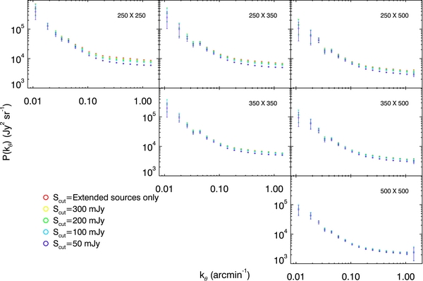
Figure 5. Spectra combined from the different fields for different levels of resolved source masking, plotted as circles with error bars. The best estimates of the cirrus spectra in each field (Section 3.3) are removed before combining. All data and uncertainties are tabulated in Table 10.
Download figure:
Standard image High-resolution imagePoisson levels are determined through a simultaneous fit to the combined spectra of the Poisson and clustered galaxy terms with templates adopted from the Viero et al. (2009) halo model, and are shown as a function of flux cut of masked sources in Figure 6 and tabulated in Table 8. We note that this estimate is subject to systematic uncertainties due to the mild degeneracy of the Poisson and 1-halo terms, more so for spectra with fewer masked sources, and that we account for those uncertainties in the estimate. As anticipated, shorter wavelengths are significantly more affected by removal of the brightest sources (see Figure 1). Previous measurements from Amblard et al. (2011) with 50 mJy sources masked are in relatively good agreement, with 250 μm higher by ∼5%, and 350 and 500 μm lower by ∼7% and 17%, respectively. The BLAST measurements, which masked sources with flux densities greater than 500 mJy (Viero et al. 2009; Hajian et al. 2012), appear to be higher than our values by ∼26%, 12%, and 11% at 250, 350, and 500 μm, respectively.
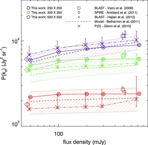
Figure 6. Poisson noise level vs. flux cut of masked sources. Best estimates of the auto-frequency spectra values are shown as open circles and tabulated in Table 8. It is worth noting that the data points between bands are not independent. Estimates of the Poisson level derived from SPIRE P(D) source counts (Glenn et al. 2010) are shown as crosses with asymmetric error bars, whose sizes are functions of the uncertain upper limits on the faint end, and that the fields studied were relatively small. Dashed lines and shaded regions represent the best estimate and 1σ uncertainties of the Béthermin et al. (2011) model, with which we find good agreement at all but 350 μm, which is underpredicted by approximately 1σ. Also shown are measured Poisson levels from BLAST (squares: Viero et al. 2009; plus signs: Hajian et al. 2012), and SPIRE (diamonds: Amblard et al. 2011).
Download figure:
Standard image High-resolution imageAlso plotted are estimates of the Poisson level derived from the Glenn et al. (2010) P(D) number counts using Equation (2). We find that the number count predictions overestimate our values by ∼16% at 250 μm, and underestimate our measured values by ∼12% and 16% at 350 and 500 μm, respectively. It should be noted that differences between different cuts in a single band are correlated, and that the shot noise levels fall within the calibration uncertainties.
Finally, we compare to the model predictions of Béthermin et al. (2011), a phenomenological model which to date is the best at reproducing the observed number counts from 15 μm to 1.1 mm. We find that the model is in very good agreement with the data at all flux-cut levels and at all but 350 μm, which underpredicts the data by approximately 1σ.
4.3. Comparison to Published Measurements
In Figure 7 we plot our combined auto-frequency power spectra along with a selection of recently published CIBA measurements. We show the two masking extremes of our data: those in which all sources greater than 50 mJy were masked (dark blue open circles), and those where only extended sources were masked (light blue open circles). We do this in order to adequately compare with the wide range of masking in the literature.

Figure 7. Comparison of our cirrus-corrected, combined data to published measurements. Data are plotted as kθP(kθ) in order to reduce the dynamic range of the plotted clustering signal, and thus better visualize the differences between the measurements. Furthermore, in order to adequately compare to the wide range of source masking found in the literature, we present the two masking extremes of our analysis: spectra with sources greater than 50 mJy masked (dark blue circles), and those with only extended sources having been masked (light blue circles). Previous SPIRE measurements from Amblard et al. (2011), which should be compared to the dark blue circles, are shown as black plus signs. The remaining data and curves should be compared to the light blue circles. Note that to help aid the comparison, error bars include systematics due to calibration and beam uncertainties. They are: BLAST data from Viero et al. (2009; brown crosses) and Hajian et al. (2012; lavender diamonds) and Planck data from Planck Collaboration et al. (2011b; red squares) at 350 and 500 μm. Note, Planck data are color corrected to account for their different passbands by multiplying the 350 and 500 μm data by factors of 0.99 and 1.30, respectively, and adjusted to the most current calibration by dividing them by 1.14 and 1.30, respectively (see Planck Collaboration et al. 2013).
Download figure:
Standard image High-resolution imageShown as black plus signs are the SPIRE auto-frequency power spectra of ∼15 deg2 from Amblard et al. (2011) in which pixels greater than 50 mJy were masked, so that they should be compared to our dark blue circles. On larger scales (e.g., kθ ≲ 0.08 arcmin−1), particularly at shorter wavelengths, their spectra suffer from overcorrection of Galactic cirrus contamination (see discussion in Planck Collaboration et al. 2011b). On smaller scales we find that our spectra differ by factors of ∼0.91 ± 0.01, 1.09 ± 0.01, and 1.09 ± 0.01. Note that the calibration of the science demonstration phase maps used in Amblard et al. (2011) differed by 1.02, 1.05, and 0.94, at 250, 350, and 500 μm, respectively, but that those corrections were not applied here. These calibration differences, combined with the offsets resulting from the new estimate of the beam (Appendix B), may partially account for this difference. Also note that although the error bars on their data are comparable to ours at small angular scales, correlations due to the non-Gaussian term (first term in Equation (5)) were not included when they rebinned into log bins, thus artificially deflating their errors.
Shown as red squares at 350 and 500 μm are results from the Planck Collaboration et al. (2011b), which should be compared to our light blue circles. Note, comparisons of the two spectra must be made with caution, bearing in mind that the flux density of masked sources in Planck is much higher (710 and 540 mJy at 350 and 550 μm). In addition, because the passbands of the two instruments are not the same, Planck data at 857 and 545 GHz (350 and 550 μm) are color corrected by multiplying them by factors of 0.99 and 1.30, respectively.
We find possible inconsistencies between the two sets of measurements. On scales kθ ≲ 0.04 arcmin−1, the Planck spectra appear to be offset high by factors of 1.26 ± 0.06 and 1.40 ± 0.06 at 350 and 500 μm, respectively, while on smaller angular scales there is an apparent excess of power in the Planck data, though it should be noted that, point by point, the 350 μm values do agree within errors. Potential explanations for this discrepancy include calibration, excess Poisson, or reconstruction systematic errors in the Planck beam. We discuss these scenarios in more detail in Section 6.2.
4.4. Comparison to Published Models
In Figure 8 we plot our combined auto-frequency power spectra next to a selection of published halo models. As in Figure 7, we show the two masking extremes of our data in order to adequately compare with the wide range of masking in the literature.

Figure 8. Comparison of our cirrus-corrected, combined data to published models. Best-fit halo models to previously published SPIRE data (Amblard et al. 2011) are shown as gray dot-dashed lines, and should be compared to the dark blue circles. The remaining curves should be compared to the light blue circles. Note, with the exception of the BLAST model (Viero et al. 2009), all of the following were originally fit to the 857 and 545 GHz channels of Planck, and have thus been color-corrected by 0.99 and 1.30 at 350 and 500 μm, respectively. They are from: Viero et al. (2009; brown dotted lines); Planck Collaboration et al. (2011b; red dashed lines) at 350 and 500 μm; case 0 of Shang et al. (2012; green dashed lines); and Xia et al. (2012; orange triple-dot-dashed lines).
Download figure:
Standard image High-resolution imageThe Viero et al. (2009) models (brown dotted lines), which were fit to BLAST data with sources greater than 500 mJy masked and appeared to be a good match to the Planck Collaboration et al. (2011b) data, here do a poor job of describing the SPIRE measurements, overestimating the power on scales greater than ∼40''.
The Amblard et al. (2011) models, which assumed a masking level of 50 mJy and were fit to each band individually, are shown as gray dot-dashed lines. Similar to the differences in the data, the large-scale power is underestimated due to the overcorrection for the contribution from Galactic cirrus, while on small scales, the small differences may be due to difference in the calibration.
The halo models from the Planck Collaboration et al. (2011b) are shown as red dashed lines at 350 and 500 μm. They assumed a masking level consistent with the masking level of Planck data, as do all following models. Their published data must be corrected for calibration by dividing them by factors of 1.14 and 1.30 at 350 and 500 μm, respectively (Planck Collaboration et al. 2013), after which they agree very well with our data.
The Xia et al. (2012) halo model, shown as orange triple-dot-dashed lines in Figure 8, was fit to Planck and corrected SPIRE data from Planck Collaboration et al. (2011b, Section 5.3). It adopts a description for the source population from Lapi et al. (2011) (an update of Granato et al. 2004). It appears to be consistent with the overall amplitude of the data, but has a bump of excess emission at around kθ ∼ 0.1–0.03 that the data do not show. This evolutionary model assumes that the steep part of the source counts at submillimeter wavelengths is dominated by massive, proto-spheroidal galaxies in the process of forming most of their stars. The model also includes small contributions from late-type and starburst galaxies. Notable in this model is that the redshift distribution of the emission peaks at slightly higher redshifts, broadly around z ∼ 1.7–2.2, increasing with increasing wavelength; this is in distinction to other models which are strongly peaked at z ∼ 1. It was fit to data from Herschel/SPIRE (Amblard et al. 2011), Planck/HFI (Planck Collaboration et al. 2011b), SPT (Shirokoff et al. 2011), and ACT (Dunkley et al. 2011), and as it is physically based, it is much more constrained than the phenomenological models used by, e.g., Viero et al. (2009) or Shang et al. (2012). That two populations are represented is evidenced by the clear feature at ∼0.2 arcmin−1, a feature which is not apparent in the data, suggesting an overestimate of the contribution of late-type galaxies to the total spectrum.
Lastly, shown as green dashed lines is the Shang et al. (2012) model, whose main feature is to implement a luminosity–mass (L–M) relation, such that more massive halos host more luminous sources. Though the model was fit primarily to Planck data, it appears to fit our spectra at 500 μm quite well. The fit is less good at 250 and 350 μm; though the shape is in good agreement, the curves are high by ∼30%. Despite this success, the model has some points of concern. In particular, it underpredicts the contribution of lower redshift sources to the CIB (e.g., they are significantly below the lower limits measured from stacking 24 μm selected sources; Jauzac et al. 2011), and we also find an uncharacteristically large β (discussed further in Section 6.3).
Finally, we highlight the feature that appears in the data at kθ ∼ 0.03–0.04 arcmin−1, particularly in all auto- and cross-frequency spectra, but predominantly at 500 μm. A similar feature was visible in the SPIRE data of Amblard et al. (2011) as well. It is not clear if this is a real feature in the sky, which would be unexpected and is unlikely, or due to noise present in the data. Similar features do not appear in the transfer function, or in the simulations of the pipeline which tested for potential biases.
4.4.1. Clustered Galaxy Power Spectra
Ultimately, we are interested in the power spectra of clustered DSFGs, which we estimate by removing the Poisson noise from the cirrus-subtracted, combined power spectra of Figure 5. Results are shown in Figure 9. The fraction anisotropy is calculated as
where ICIB is the overall amplitude of the CIB, measured to be 0.71 ± 0.17, 0.59 ± 0.14, and 0.38 ± 0.10 MJy sr−1 at 250, 350, and 500 μm, respectively (e.g., Lagache et al. 2000; Marsden et al. 2009), and kθ is converted to sr. We find δI/I = 14% ± 4%, consistent with findings from Viero et al. (2009).

Figure 9. Combined clustering spectra vs. flux-cut level of masked sources. Spectra are shifted horizontally for visual clarity. Overlaid are best-fit templates to the data from our Model 3 (Section 5). If resolved sources contributed solely to the Poisson noise component of the spectra, then these points would lie on top of one another. Instead, there is a clear reduction of 1-halo power with masking level at 250 μm, suggesting that some fraction of bright DSFGs are either close pairs or reside, as satellites, in more massive dark matter halos.
Download figure:
Standard image High-resolution imageWe fit a simple power law to the clustering spectra over the range kθ = 0.01–1.4 arcmin−1, finding a mild change in the slope with changes in the masking level. Specifically, from most (Scut > 50 mJy) to least aggressively masked (only extended sources), we find slopes of −1.60 ± 0.05 to −1.50 ± 0.07 at 250 μm, −1.52 ± 0.05 to −1.36 ± 0.06 at 350 μm, and −1.52 ± 0.06 to −1.47 ± 0.06 at 500 μm. The χ2 of these fits for 15 degrees of freedom (dof) are 7, 10, and 3 (reduced χ2 ∼ 0.5, 0.7, and 0.3) at 250, 350, and 500 μm, respectively.
The next notable feature is the reduction of 1-halo power with flux cut of masked sources, particularly at 250 μm, which is shown as dashed lines in Figure 9, whereas the 2-halo power, shown as dotted lines, remains relatively unchanged. We demonstrate in Section 6.1 how this result can be interpreted as more luminous sources residing in more massive halos, motivating the use of a model later in the paper in which an L–M relationship is invoked (e.g., Sheth 2005; Skibba et al. 2006; Shang et al. 2012). We show that attempting to account for the reduction of power entirely with the Poisson term leads to significant tension in the fit. Though the reduction of power is much less significant at 500 μm, we remind the reader that there are far fewer sources at each given flux-cut level at 500 μm than at 250 or 350 μm (see Table 2). The capability to mask fainter sources reliably at 500 μm would require either maps with higher angular resolution (i.e., less confusion noise) or a way to probe deeper into the confusion using ancillary data (e.g., XID; Roseboom et al. 2010).
4.5. Cross-correlation Power Spectra
The cross-correlation power spectrum is defined as
i.e., the ratio of the cross-frequency power spectra to the geometric mean of the two auto-frequency power spectra. Identical maps would thus have a cross-correlation of unit amplitude, as would maps containing sources located at identical redshifts and with identical colors. Departures from unity would be an indication that sources are not all at the same redshift, or that their colors (or average temperatures) are variable, and the strength and shape of the cross-correlation signal would depend on the level of correlation between maps. Consequently, the cross-correlation provides strong constraints for source population models.
We show the cross-correlations as functions of the flux cut of masked sources in Figure 10. The measurement becomes very uncertain at angular scales kθ ⩽ 0.1 arcmin−1. At larger kθ, with the exception of the 50 mJy cut, we find similar levels of correlation for all levels of masking, which can be approximated as horizontal lines at 0.95 ± 0.04, 0.86 ± 0.04, and 0.95 ± 0.03 for A × B = 250 × 350, 250 × 500, and 350 × 500, respectively. Cross-correlations of maps with sources masked at 50 mJy appear to be less correlated, with hints of a reduction in the correlation with increasing kθ, which, as first predicted by Knox et al. (2001), would be an indication that longer wavelengths are more sensitive to higher z.
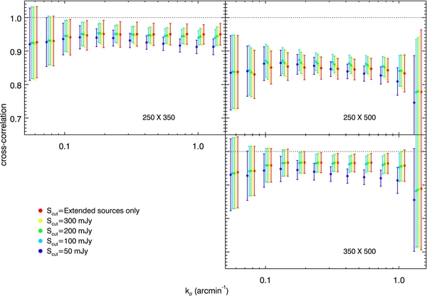
Figure 10. Cross-correlation power spectra. Spectra are shifted horizontally for visual clarity. For two identical maps, or two maps in which all the sources are at the same redshift, this measurement would have unit amplitude, which is represented by a dotted line. We find that for unmasked maps, the cross-correlation is approximately 0.95 ± 0.04, 0.86 ± 0.04, and 0.95 ± 0.03 for 250 × 350, 250 × 500, and 350 × 500, respectively. For maps with sources greater than 50 mJy masked, this cross-correlation is reduced, and appears to weaken further with decreasing angular scale.
Download figure:
Standard image High-resolution imageThese results compare favorably with the Planck Collaboration et al. (2011b) measurements of the cross-correlation, who found 0.89 and 0.91 for two different fields at 350 × 550 μm, and are also consistent within errors with the cross-correlations measured by Hajian et al. (2012).
5. HALO MODEL INTERPRETATION OF CIB ANISOTROPY MEASUREMENTS
The angular power spectrum of intensity fluctuations,  , is obtained using Limber's approximation (Limber 1953), which is valid on small angular scales (2πkθ ≳ 10). The projection of the flux-weighted spatial power spectrum is
where χ(z) is the comoving distance to redshift z, and dSν/dz is the redshift distribution of the cumulative flux. The redshift range used here is 0 < z < 4, from which most of the CIB is emitted (e.g., Béthermin et al. 2012a). For sources with flux densities Sν ⩽ Scut
and the differential number counts are related to the epoch-dependent comoving luminosity function, dn/dL(L, z), through
5.1. Halo Model Formalism
The power spectrum of CIBA in the halo model formalism is written as the sum of three terms: the linear (or 2-halo) term, which accounts for pairs of galaxies in separate halos and dominates the spectrum on large scales; the nonlinear (or 1-halo) term, which describes pairs of galaxies residing in the same halo and is the dominant term on small scales; and the Poisson (or shot) noise term:

Common to most halo models is that a distinction is made between central and satellite galaxies, with Ngal = Ncen + Nsat. All halos above a minimum mass Mmin host a galaxy at their center,
while any additional galaxies in the same halo would be designated as satellites which trace the dark matter density profile (e.g., Zheng et al. 2005). Halos host satellites when their mass exceeds the pivot mass M1 (also known as Msat in the literature), and the number of satellites is an exponential function of halo mass:
In earlier halo models, galaxies were assumed to contribute equally to the emissivity density (e.g., Viero et al. 2009; Amblard et al. 2011; Planck Collaboration et al. 2011b). Therefore, assuming that the CIB originates from galaxies, spatial variations in the specific emission coefficient jν directly trace fluctuations in the galaxy number density

The linear, 2-halo term dominates on large scales and is given by the clustering of galaxies in separate dark matter halos:
with
where Plin(k, z) is the linear dark matter power spectrum, b(M, z) is the linear large-scale bias, and ugal(k, z, M) is the normalized Fourier transform of the galaxy density distribution within a halo, which is assumed to equal the dark matter density profile, i.e., ugal(k, z, M) = uDM(k, z, M). The nonlinear, 1-halo term dominates on small scales, and is written as
(Cooray & Sheth 2002), where dN/dM is the halo mass function.
However, conceptually it is wrong to assume that galaxies of different luminosities have equal weight in contributing to the power spectrum of the intensity fluctuations. A consequence of this assumption is that the excess signal on small angular scales from galaxies in massive halos can only be reproduced by having more satellite galaxies, leading to previous estimates of α which exceed predictions for subhalo indices from semi-analytic models (α ⩽ 1; e.g., Gao et al. 2004; Hansen et al. 2009) and a significant overabundance of satellites. For example, previous halo model fits to SPIRE data from Amblard et al. (2011) found α ∼ 1.7 at 250 μm and ∼1.8 at 350 and 500 μm, albeit with large errors.
A way to overcome this excess satellite problem, while still producing enough 1-halo power, is to have a model with fewer but more luminous satellites and weight galaxies by their luminosities. One such model is that of Shang et al. (2012), which invokes an L–M relation to tie the emissivity from galaxies to their host halo masses (also see, e.g., Yang et al. 2003; Vale & Ostriker 2004). The advantage of this model is that in principle one can predict the abundance as well as the clustering of galaxies observed at different frequency bands simultaneously, while in previous halo models it was impossible to predict the power spectrum across different frequency bands at the same time. As we will now show, this new formalism is similar to previous ones up until the numbers of central and satellite galaxies are substituted for luminosity-weighted quantities.
5.2. Luminosity-Weighted Halo Model
Hereafter, we follow the formalism of Shang et al. (2012), with some modifications. Novel to our implementation is the simultaneous fitting to the power spectra in all three bands, and to the number counts of sources above about 0.1 mJy (Glenn et al. 2010). In this implementation of the halo model, the mean comoving specific emission coefficient is
where L is the luminosity and dn/dL is the luminosity function of DSFGs. What this means is that, unlike the earlier models, which assume that all galaxies contribute equally to the emissivity density (i.e., have the same luminosity), here the emissivities of galaxies in a given halo, by way of their luminosities, depend on the redshift, halo mass, and frequency:

where L0 is the overall normalization factor, η describes the redshift evolution, Σ(M) describes the relation between infrared luminosity and halo mass (the L–M relation), and Θ(v) describes the shape of the infrared SED. Note that here M represents both the mass of the main halo and the infall mass of the subhalo.
Furthermore, the effective, luminosity-weighted number of central and satellite galaxies is
where dn/dm(M, z) is the subhalo mass function of the main halo whose mass is M.
The terms in Equations (23) and (24) remain the same, except the numbers of central and satellite galaxies are substituted with their luminosity-weighted counterparts, such that Dν in the 2-halo term (Equation (23)) becomes
and the 1-halo term (Equation (24)) becomes
We define halos here as overdense regions whose mean density is 200 times the mean background density of the universe according to the spherical collapse model, and we adopt the density profile of Navarro et al. (1997) with the concentration parameter of Bullock et al. (2001), and the fitting function of Tinker et al. (2008) for the halo mass function and its associated prescription for the halo bias (Tinker et al. 2010). For the subhalo mass function, we use the fitting function of Tinker & Wetzel (2010). We will now describe each of the terms in Equation (26) in more detail. Note that using instead the concentration parameter of Duffy et al. (2008) leads to very little change in the final best-fit parameters.
5.2.1. (1 + z)η: The Luminosity Evolution
The luminosity evolution in this model is motivated by the known increase of specific star formation rate (sSFR) with redshift (e.g., Elbaz et al. 2007; Oliver et al. 2010a; Karim et al. 2011; Noeske et al. 2007; Sargent et al. 2012; Wang et al. 2012), and the fact that SFRs and infrared luminosities are correlated for DSFGs (e.g., Kennicutt 1998). The exact form of the evolution is still not clear: though measurements find a rapid rise followed by plateau at z ≳ 2 (e.g., Stark et al. 2009; González et al. 2010), semi-analytic models have difficultly reproducing observations without invoking a number of ad hoc modifications to the standard physical recipes (e.g., Weinmann et al. 2011). Yet, without a convincing alternative, we proceed motivated by observations, letting η be a free parameter over 0 < z < 2 and setting η = 0 at z ⩾ 2.
5.2.2. Σ(M): The L–M Relation
Observationally it is clear that some halos are more efficient than others at hosting star formation (e.g., Béthermin et al. 2012b; Wang et al. 2012), and that the halo mass of most efficient star formation evolves with redshift (i.e., downsizing; e.g., Cowie et al. 1996; Bundy et al. 2006). It is also clear that star formation in halos is suppressed by several plausible mechanisms at the high-mass (e.g., accreting black holes; Birnboim & Dekel 2003; Kereš et al. 2005) and low-mass (e.g., feedback from supernovae, photoionization heating; Dekel & Silk 1986; Thoul & Weinberg 1996) extremes. Thus, following Shang et al. (2012), we assume that the L–M relation, Σ(m), can be parameterized by a simple log-normal distribution
where Mpeak describes the peak of the specific IR emissivity per unit mass, and  describes the range of halo masses in which galaxies producing IR emission reside. The minimum halo mass to host a galaxy, Mmin, is left as a free parameter, but we place a lower limit on it such that L = 0 at M < Mmin.
Note that we have implicitly assumed that the shape of the relation between halo mass and infrared luminosity is redshift-independent and identical for both central and satellite galaxies. Equation (25) can then be recast as
where m is the subhalo mass at the time of accretion (e.g., Wetzel & White 2010; Shang et al. 2012) and dn/dm is the subhalo mass function in a host halo of mass M at a given redshift.
5.2.3. Θ(ν): The Model SED
Following Hall et al. (2010) and Shang et al. (2012), we begin with the simplest model SED, a single modified blackbody:

where B(ν, Td) is the blackbody spectrum (or Planck function), with effective dust temperature Td, and β is the emissivity index. Both Td and β are free variables with no redshift evolution. We refer to this as Model 1.
Next, in attempting to address the growing observational evidence for evolving temperature with redshift (e.g., Pascale et al. 2009; Amblard et al. 2010; Viero et al. 2013), we introduce an additional parameter, Tz, such that  . Note that the β parameter remains a free variable without redshift evolution in this model, which we refer to as Model 2.
Lastly, motivated by the findings of, e.g., Dunne & Eales (2001) or Elbaz et al. (2011)—who found that a typical DSFG spectrum is better fit by a linear combination of two SEDs: (1) those from hotter (Td, warm ∼ 50 K), star-forming regions, and (2) those from colder (Td, cold ∼ 20 K) regions of diffuse interstellar medium—we adopt a two-component SED. The ratio of the masses in the two components is defined as ξ =log(Nc/Nw), and is independent of redshift. Here β is redshift independent and fixed to equal 2. We refer to this model as Model 3.
5.2.4. Markov Chain Monte Carlo
We make use of Markov Chain Monte Carlo methods to derive the posterior probability distributions for all parameters by fitting to the P(D) number counts (Glenn et al. 2010) and all auto- and cross-frequency power spectra at 250, 350 and 500 μm simultaneously. Further, fits are performed simultaneously to spectra with sources above 50 and 300 mJy masked. Finally, the absolute CIB as measured by Lagache et al. (2000; 10.4 ± 2.3, 6.5 ± 1.6, 2.6 ± 0.6 nW m−2 sr−1) provides additional constraints.
Models 1, 2, and 3 consist of seven, eight, and nine free parameters, respectively. All models include: one for the low-mass halo cutoff (Mmin), two for the L–M relation (Mpeak and σL/m), one for the redshift evolution (η), and an overall normalization (L0). Models 1 and 2 have two parameters for the SED (Td and β), while Model 3 has two SED temperature parameters (Tcold and Twarm) and a parameter describing the ratio of the masses in the two components (ξ). Lastly, Models 2 and 3 have parameters to describe the evolution of the dust temperature with redshift (Tz).
5.3. Halo Model Results
The best-fit parameters for Models 1, 2, and 3 are tabulated in Tables 4, 5, and 6, respectively, and shown in Figure 11. The respective best fits to the counts are shown in Figure 12. The corresponding χ2 (dof) are 368 (225), 357 (224), and 371 (223), or  , 1.6, and 1.7, for Models 1, 2, and 3, respectively. That the addition of a parameter does not significantly improve the fits is discussed in Section 6.3.
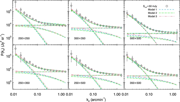
Figure 11. Best-fit halo models fit simultaneously to cirrus-subtracted, combined auto- and cross-frequency power spectra (with sources greater than Scut = 50 mJy masked) and to the P(D) number counts from Glenn et al. (2010). Spectra are fit with three terms: Poisson (horizontal lines), 2-halo (steep lines dominant at low kθ), and 1-halo (less steep and contributing at all kθ). The sum of the three terms is also plotted.
Download figure:
Standard image High-resolution image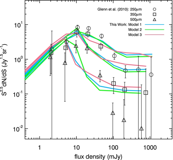
Figure 12. Euclidean normalized differential number counts from Glenn et al. (2010, shown as circles, squares, and triangles at 250, 350, and 500 μm, respectively) along with best-fit curves from the three models. These curves were found by simultaneously fitting to spectra (shown in Figure 11) as well as to these counts. This fit reveals a possible tension between the modeling of the counts and the modeling of the clustering terms.
Download figure:
Standard image High-resolution imageTable 4. Model 1: Best-fit Parameters and Corresponding Correlation Matrix
| Parameter | log(Mmin) | log(Mpeak) | T | β |  |
log(L0) | η |
|---|---|---|---|---|---|---|---|
| log(Mmin) | 9.8 ± 0.5 | 0.16 | −0.09 | 0.06 | −0.15 | −0.23 | 0.23 |
| log(Mpeak) | ... | 12.2 ± 0.5 | −0.11 | 0.16 | −1.00 | −0.42 | 0.49 |
| T | ... | ... | 23.1 ± 1.3 | −0.97 | 0.10 | 0.74 | −0.29 |
| β | ... | ... | ... | 1.4 ± 0.1 | −0.16 | −0.62 | 0.25 |
 |
... | ... | ... | ... | 0.4 ± 0.0 | 0.41 | −0.50 |
| log(L0) | ... | ... | ... | ... | ... | −1.7 ± 0.1 | −0.74 |
| η | ... | ... | ... | ... | ... | ... | 2.0 ± 0.1 |
Notes. Best-fit parameters and correlations between them in Model 1. Off-diagonal values of +1 or −1 mean that the parameters are highly correlated or anti-correlated, respectively, while values near 0 mean that they are independent of one another.
Download table as: ASCIITypeset image
Table 5. Model 2: Best-fit Parameters and Corresponding Correlation Matrix
| Parameter | log(Mmin) | log(Mpeak) | T | Tz | β |  |
log(L0) | η |
|---|---|---|---|---|---|---|---|---|
| log(Mmin) | 10.1 ± 0.5 | −0.02 | 0.20 | −0.27 | −0.10 | 0.02 | 0.26 | −0.25 |
| log(Mpeak) | ... | 12.3 ± 0.5 | 0.21 | −0.01 | −0.23 | −1.00 | −0.18 | 0.20 |
| T | ... | ... | 20.7 ± 1.2 | −0.66 | −0.92 | −0.21 | 0.76 | −0.56 |
| Tz | ... | ... | ... | 0.2 ± 0.0 | 0.38 | 0.01 | −0.81 | 0.89 |
| β | ... | ... | ... | ... | 1.6 ± 0.1 | 0.23 | −0.53 | 0.31 |
 |
... | ... | ... | ... | ... | 0.3 ± 0.0 | 0.18 | −0.20 |
| log(L0) | ... | ... | ... | ... | ... | ... | −1.8 ± 0.1 | −0.90 |
| η | ... | ... | ... | ... | ... | ... | ... | 2.4 ± 0.1 |
Notes. Best-fit parameters and correlations between them in Model 2. Off-diagonal values of +1 or −1 mean that the parameters are highly correlated or anti-correlated, respectively, while values near 0 mean that they are independent of one another.
Download table as: ASCIITypeset image
Table 6. Model 3: Best-fit Parameters and Corresponding Correlation Matrix
| Parameter | log(Mmin) | log(Mpeak) | Twarm | Tcold | ξ | Tz |  |
log(L0) | η |
|---|---|---|---|---|---|---|---|---|---|
| log(Mmin) | 10.1 ± 0.6 | −0.39 | 0.40 | 0.40 | −0.23 | −0.43 | 0.39 | 0.42 | −0.41 |
| log(Mpeak) | ... | 12.1 ± 0.5 | −0.75 | −0.91 | 0.02 | 0.89 | −1.00 | −0.79 | 0.90 |
| Twarm | ... | ... | 26.6 ± 2.8 | 0.80 | −0.05 | −0.90 | 0.75 | 0.94 | −0.90 |
| Tcold | ... | ... | ... | 14.2 ± 1.0 | 0.05 | −0.93 | 0.90 | 0.80 | −0.92 |
| ξ | ... | ... | ... | ... | 1.8 ± 0.1 | 0.18 | −0.02 | −0.27 | 0.19 |
| Tz | ... | ... | ... | ... | ... | 0.4 ± 0.1 | −0.88 | −0.95 | 0.99 |
 |
... | ... | ... | ... | ... | ... | 0.4 ± 0.0 | 0.79 | −0.89 |
| log(L0) | ... | ... | ... | ... | ... | ... | ... | −1.9 ± 0.1 | −0.96 |
| η | ... | ... | ... | ... | ... | ... | ... | ... | 2.7 ± 0.2 |
Notes. Best-fit parameters and correlations between them in Model 3. Here ξ is the ratio of the masses of the cold and warm components. Off-diagonal values of +1 or −1 mean that the parameters are highly correlated or anti-correlated, respectively, while values near 0 mean that they are independent of one another.
Download table as: ASCIITypeset image
Correlations between parameters are presented in the off-diagonal entries of Tables 4, 5, and 6 for Models 1, 2, and 3, respectively. As pointed out by, e.g., Shang et al. (2012), certain pairs of parameters exhibit very high levels of correlation: in particular, the SED parameters (β and T in Models 1 and 2, Tcold and Twarm in Model 3), the luminosity parameters η and L0, and the mass parameters  .
.
We find that star formation is most efficient in halos ranging from log(M☉) = 11.7 to 12.5, peaking at log(M☉) ∼ 12.1, which is consistent with several recent results from observations and simulations (e.g., Moster et al. 2010; Wang et al. 2012; Behroozi et al. 2013). In Cooray et al. (2010), where a halo model is developed to fit the angular correlation functions of galaxies brighter than 30 mJy, the minimum halo mass scale is log (Mmin/M☉) = 12.6, 12.9, and 13.5 at 250, 350, and 500 μm, respectively. These values are much higher than our best-fit log (Mmin/M☉) = 10.1 ± 0.6, which is due to the fact that faint galaxies (around 5 mJy) dominate the power spectrum of the intensity fluctuations (see Figure 1). In Amblard et al. (2011), the minimum halo mass scale is log (Mmin/M☉) = 11.1, 11.5, and 11.8 at 250, 350, and 500 μm, respectively, which are higher than our best-fit value. Furthermore, the evolution of the dust temperature, characterized by Tz, is in very good agreement with stacking measurements found by, e.g., Pascale et al. (2009) and Viero et al. (2013).
The redshift distribution of the emissivity—which in previous halo models has been either parameterized or adopted from galaxy population models—is here an output of the L–M relation, and shown compared to a selection of models (Valiante et al. 2009; Béthermin et al. 2011, 2012a) and previous estimates (Amblard et al. 2011) in Figure 13.
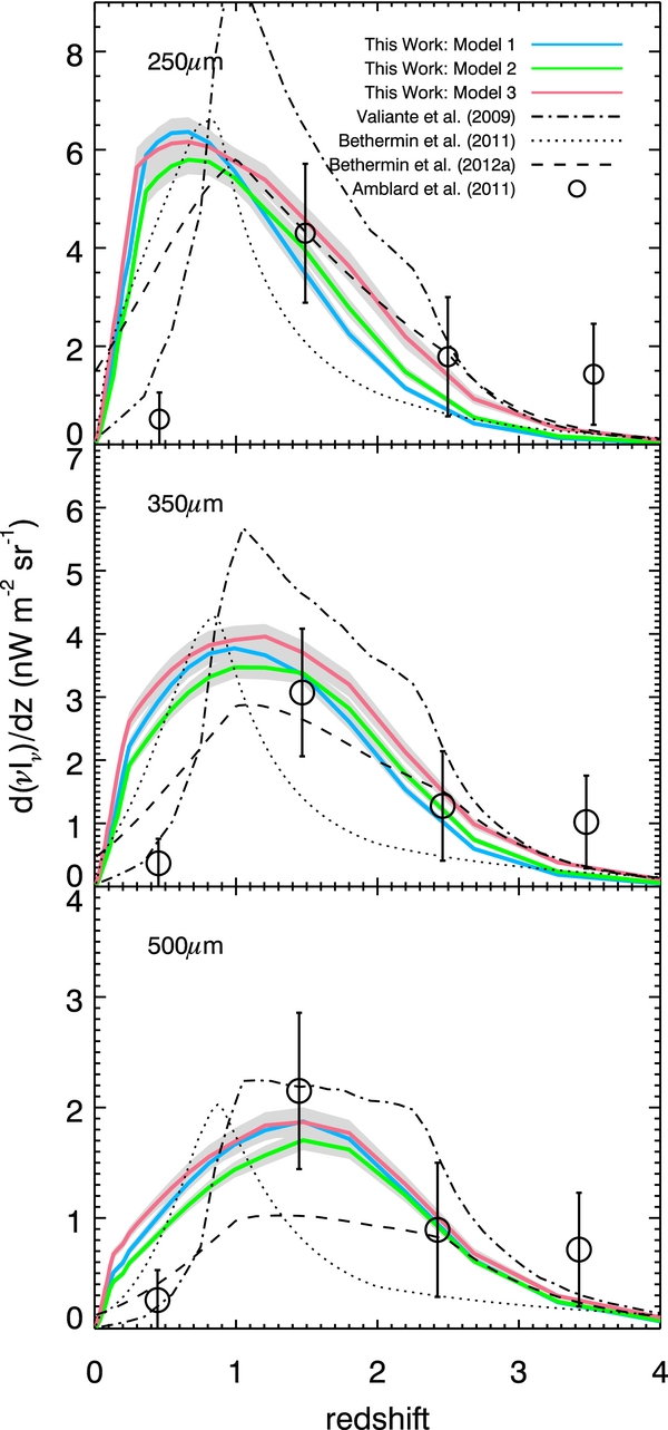
Figure 13. Redshift distribution of emission for Models 1, 2, and 3. The Amblard et al. (2011) points were estimated in a similar manner, finding the best-fit solution to their power spectra with a halo model. The model predictions of Béthermin et al. (2011) and Béthermin et al. (2012a) are shown as dotted and dashed lines, respectively. Also shown are model predictions from Valiante et al. (2009). The models unanimously anticipate more of a contribution from z ≳ 2 than our best fit finds.
Download figure:
Standard image High-resolution imageLastly, we plot the absolute CIB in each band output by our model, along with several measurements from the literature, in Figure 14. We find that our models are consistent with the fiducial FIRAS values (Fixsen et al. 1998; Lagache et al. 2000), though we note that the uncertainties in the fiducial measurements are of order 30%.
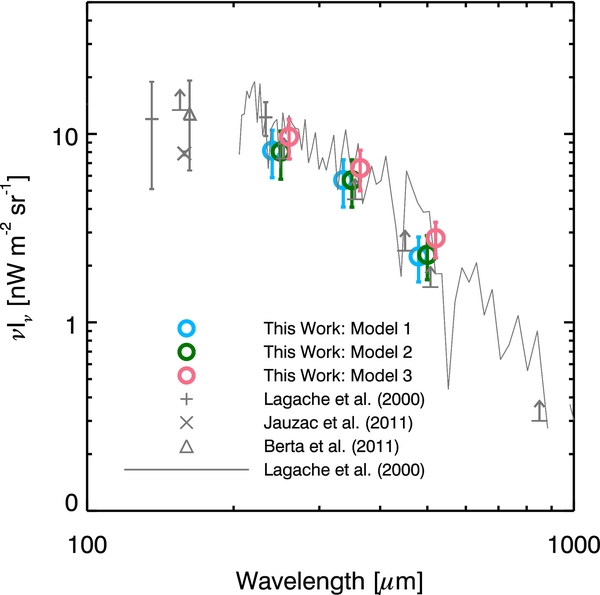
Figure 14. Integrated CIB from Models 1, 2, and 3 is plotted as colored circles, along with a selection of measurements of the total CIB in gray, including: 160 μm with Herschel/PACS from Jauzac et al. (2011; cross) and Berta et al. (2011; triangle), 140 and 240 μm with WHAM from Lagache et al. (2000; plus signs), and ∼200 to 1200 μm spectra with COBE/FIRAS from Lagache et al. (2000; solid line). Lower limits are from SPIRE at 250, 350, and 500 μm (Béthermin et al. 2012c) and SCUBA at 450 and 850 μm (Smail et al. 2002; Serjeant et al. 2004).
Download figure:
Standard image High-resolution image6. DISCUSSION
We find a clear signature from the clustering of DSFGs in the pattern of CIBA, with the fidelity to identify linear and nonlinear terms. Notable is how well the spectra are still fit by a power law, with χ2 ∼ 3–10 for 15 dof (reduced χ2 ∼ 0.3–0.7)—a cosmic coincidence first seen in early clustering measurements of resolved galaxies (e.g., Watson et al. 2011). Future measurements on larger scales, which should bracket the expected peak of the linear, 2-halo spectra, will eventually rule out the power law as a viable fit. That the halo model is well motivated regardless is evidenced by the change in the power spectrum with changes in the level of source masking: while it appears that the 2-halo term is negligibly affected, the 1-halo term is significantly reduced. We now discuss plausible interpretations of this reduction in power.
6.1. The Reduction of 1-Halo Power with Masking
Since the 1-halo term originates from multiple galaxies occupying the same halo, the reduction of the 1-halo term with more aggressive source masking suggests that some fraction of the more luminous resolved SPIRE sources are satellites in massive halos or cluster members, though it should be noted that some fraction of bright galaxies could be close pairs, which would make the same imprint on the spectra. This is consistent with the interpretation from clustering measurements of resolved SPIRE sources which claims that ∼14% of sources with S250 > 30 mJy appear as satellites (Cooray et al. 2010).
One may wonder if the reduction in power can be solely attributed to a reduction in the Poisson level, but this is unlikely. We show this by fitting the unmasked 250 μm spectra with a 2-halo, 1-halo, and Poisson term, and then fitting the same terms to spectra with sources above 50 mJy masked. The 2-halo term is fixed in both for both levels of masking, while in the latter fit the 1-halo term is first fixed and then allowed to float, in order that the two fits can be compared. For a floating 1-halo term, χ2 = 10.0 for 15 dof ( ), while for a fixed 1-halo term χ2 = 98.3 for 16 dof (
 ), thus ruling out the possibility that the 1-halo term has not been affected by masking.
That some fraction of more luminous sources are found in satellite halos is also expected from semi-analytic models of DSFGs. For example, González et al. (2011) predict that 38% of all DSFGs (defined there as S ≳ 1 mJy at 850 μm) and 24% of the most luminous sources (S ≳ 5 mJy at 850 μm) are satellites. Furthermore, observations of individual groups and clusters universally find that when star-forming galaxies are present they are located on the outskirts of the massive halos (typically defined as the volume between R500 and R200; e.g., Saintonge et al. 2008; Tran et al. 2009; Braglia et al. 2011). Even more support for this scenario comes from stacking in the submillimeter at positions of brightest cluster galaxies, which shows a bump in emission at 0.8 Mpc from the central galaxy (Coppin et al. 2011). In light of these observations, the reduction of 1-halo power with masking is unsurprising.
6.2. Comparison with Planck
Released to the archive at about the same time, initial CIBA power spectra from Herschel/SPIRE (Amblard et al. 2011) and Planck/HFI (Planck Collaboration et al. 2011b) were found to be discrepant by more than 15%. The updated, published Planck Collaboration et al. (2011b) paper explored this difference in detail by comparing to power spectra of SPIRE maps that have had no masking applied (rather than the published spectra which masked all pixels greater than 50 mJy). They found that a discrepancy still remained, with SPIRE measurements lower by factors of ∼1.7 and ∼1.2 at 857 and 545 GHz (350 and 550 μm) over the angular range 0.02 < kθ/arcmin < 0.07 (400 < ℓ < 1500). If we compare our spectra, having only masked extended sources, to the Planck/HFI spectra over the same angular range, we find our spectra are also low, but by factors of ∼1.3 ± 0.06 and 1.4 ± 0.06 at 350 and 500 μm, respectively.
They next proposed a way to resolve the discrepancy. They showed that the spectra of the two groups could be brought into agreement if: (1) no Galactic cirrus is removed from the SPIRE data; and (2) the beam surface area—which they claim to be overestimated by ∼4% and 9% at 350 and 500 μm, respectively—is corrected. Indeed, we also find that the previous cirrus values were overestimated; and from a careful estimate of the beam area (described in detail in Appendix B), we also find a correction, though equaling ∼2% and 8%. These corrections have brought the overall offset, particularly on scales kθ ≲ 0.04 arcmin−1 (ℓ ≲ 900), into agreement; however, on small scales they have been unable to close the gap entirely. The remaining offset on the largest scales can be attributed to systematic calibration uncertainties of the two instruments: 7% for SPIRE (Appendix B), and 7% for Planck/HFI (Planck Collaboration et al. 2011a), which may be a product of the very different calibration strategies of the two instruments, as well as potential systematic uncertainties from cirrus removal. But it is on scales kθ ≳ 0.04 arcmin−1 (ℓ ≳ 900)—scales on which the contribution from Galactic cirrus is negligible—that excess powers in the Planck curves are still either in tension (350 μm) or do not agree (500 μm).
Ultimately, since this paper first appeared it was determined that the Planck calibration of the 857 and 545 GHz (350 and 550 μm, respectively) channels was off by 7% and 15%, meaning that to properly compare the data their spectra must be divided by 1.14 and 1.30 (see Planck Collaboration et al. 2013). This correction—which has been applied to the data in Figure 7—indeed brings the two curves into generally good agreement.
6.3. Interpreting Halo Model Results
Our halo models represent a step forward by being the first to fit the auto- and cross-frequency power spectra, number counts, and absolute CIB levels simultaneously. The added complexity introduced by these models is justified as simpler halo models have been unable to simultaneously fit published power spectra (e.g., Planck Collaboration et al. 2011b). Yet, considering the wide range of data fit, our models remain relatively simple; e.g., they have a comparable number of parameters to the model presented in Amblard et al. (2011, which varied the Poisson level, Mmin, M1, α, and 4 dS/dz nodes, but fit each spectra independently and had no L–M relation). However, with reduced χ2 of ∼1.6, our models cannot formally be claimed to be good fits, and in fact there are some obvious problems with these models.
Firstly, the addition of parameters only marginally improves the fits, if at all. This is because the χ2 is dominated by the poor fit to the counts, particularly at the bright end (i.e., S ≳ 20 mJy). Considering that the clustering power is dominated by the sources below that flux density level (Figure 1), this tension between the fits to the counts and the fits to the spectra is not terribly surprising. It may be that this tension is attributable to there being two types of submillimeter-emitting galaxies (i.e., hotter "starburst" type galaxies, and more "normal main sequence" galaxies; e.g., Elbaz et al. 2011). Though we explore the possibility of two populations in Model 3, we do not decouple their contributions in redshift. If local starbursts are indeed responsible for a separate, lower redshift nonlinear term, then our model would struggle to satisfy the linear and nonlinear components at all redshifts, as it appears to do.
Second, there are significant degeneracies, as well as possibly questionable assumptions, built into this model. The strong coupling of the SED parameters T, β, and temperature evolution Tz renders the resulting best-fit parameters difficult to meaningfully interpret. Also, the very strong anti-correlation of luminosity evolution η and normalization L0 likewise makes interpreting the evolution of the galaxy luminosity or galaxy bias difficult. Furthermore, the assumption that the luminosity evolution increases to z = 2 and then abruptly flattens, though seen in several observations (e.g., Stark et al. 2009; González et al. 2010), is likely to be extreme and prone to galaxy selection effects (e.g., Weinmann et al. 2011). Getting this wrong would result in compensating for the discrepant high-z power by the other parameters in unpredictable ways. Lastly, the observed quenching of star formation in the cores of the most massive halos (e.g., Cattaneo et al. 2006) is not treated by the model, but may have a significant impact on the nonlinear component of the power spectrum.
Thus, our model is far from the final say in the interpretation of CIBA, as it appears that the quality of the data demands a model with additional levels of sophistication. Future models can address many of these limitations by carefully implementing observations. For example, strong constraints on the stellar-mass to halo-mass relationship (e.g., Behroozi et al. 2013), star-formation to halo-mass relationship (e.g., Wang et al. 2012), and infrared luminosity to stellar-mass relationship (Viero et al. 2013) now exist. That, combined with knowledge of the quiescent fraction of galaxies with redshift (e.g., Quadri et al. 2012), would result in more constrained models with fewer parameters. Furthermore, future models could be extended to fit not only the three SPIRE bands, but also longer wavelength data from, e.g., ACT, Planck, and SPT, as well as at shorter wavelengths from, e.g., Spitzer, IRAS, and WISE. By combining long-wavelength multi-band studies of map-based power spectra with discrete object correlations at shorter wavelengths, we should be able to build a much more complete picture of the relationship between stars, star formation, and dark matter halos.
7. SUMMARY
We have presented the auto- and cross-frequency power spectra of cosmic infrared background anisotropies at 250, 350, and 500 μm. The background originates from all of the DSFGs in the sky, i.e., those which are bright and resolved, as well as those too faint to be resolved.
We found an unambiguous signature from the clustering of DSFGs in the pattern of the background light and showed that it can be decomposed into linear (or 2-halo) power from galaxies in separate halos and nonlinear (1-halo) power from multiple central and satellite galaxies occupying massive halos. We masked resolved sources in stages down to 50 mJy and found an expected reduction in the level of Poisson noise, as well as a reduction in the 1-halo power. We interpreted the reduction in 1-halo power as resulting from some fraction of the most luminous sources being satellite galaxies. We also measured the cross-correlation of the signal between bands and found maps with more aggressive masking to be less correlated, as well as hints of a decreasing correlation with decreasing angular scale, which would be indications of decreased correlations between maps for higher-z sources.
We then attempted to interpret the measurement through the framework of the halo model, building upon and extending the formalism of Shang et al. (2012). Our models were able to simultaneously fit the auto- and cross-frequency power spectra, as well as measured number counts and absolute CIB levels from the literature. We found that, in this framework of these models, the minimum halo mass to host star formation is log(Mmin/M☉) ∼ 10.1 ± 0.6, and that star formation is most efficient in a range of halo masses centered around log(Mpeak/M☉) ∼ 12.1 ± 0.5 and  , which is in agreement with other estimates from the literature.
Our measurement has limited power to constrain angular scales kθ ≲ 0.2 arcmin−1, due partly to the relatively small areas of the individual fields, but mostly the result of the filtering performed by the SMAP pipeline. The situation will improve dramatically with the arrival of HeLMS, which was designed to constrain the turnover of the linear term by targeting the largest modes in the sky, as well as future measurements from H-ATLAS (Eales et al. 2010) and Planck. Adding to that cross-frequency correlations over the full range of angular scales from, e.g., ACT × SPIRE and SPT × SPIRE, and even Planck × Planck, which will provide powerful new constraints for models of galaxy evolution, the future indeed holds still more breakthroughs.
We thank Aurélien Benoit-Levy, Kevin Blagrave, Olivier Doré, Duncan Hanson, Amir Hajian, Peter Martin, Mattia Negrello, Aurelie Pénin, Anthony Pullen, and Christian Reichardt for valuable discussions. We also thank Olivier Doré, Cien Shang, and Jun-Qing Xia for kindly providing their halo model curves. Finally, we sincerely thank the referee for helping improve this paper considerably.
L.W. acknowledges support from UK's Science and Technology Facilities Council grant ST/F002858/1 and an ERC StG grant (DEGAS-259586). SPIRE has been developed by a consortium of institutes led by Cardiff Univ. (UK) and including: Univ. Lethbridge (Canada); NAOC (China); CEA, LAM (France); IFSI, Univ. Padua (Italy); IAC (Spain); Stockholm Observatory (Sweden); Imperial College London, RAL, UCL-MSSL, UKATC, Univ. Sussex (UK); and Caltech, JPL, NHSC, Univ. Colorado (USA). This development has been supported by national funding agencies: CSA (Canada); NAOC (China); CEA, CNES, CNRS (France); ASI (Italy); MCINN (Spain); SNSB (Sweden); STFC, UKSA (UK); and NASA (USA).
APPENDIX A: THE UPDATED SMAP PIPELINE
The reduction and map-making algorithms used with HerMES data have evolved since the description presented in Levenson et al. (2010). We review the modifications to the SMAP pipeline which lead to the DR1 (first data release) HerMES maps in this Appendix. These maps are available for download from HeDaM.38
Initial processing for the SMAP pipeline uses the Herschel Interactive Processing Environment (HIPE). For HerMES DR1, the HCSS/HIPE user release version 6.0.3, corresponding to continuous integration build 6.0.2055, was used (Ott et al. 2006; Ott 2010), including calibration tree version spire_cal_6_1. The processing script calls the Spire Photometer Interactive Analysis (SPIA; Schulz 2011) version 1.2.
In summary, the basic pipeline processing steps that are performed by HIPE are, in order:
- 1.Signal jump detection.
- 2.Common glitch detection.
- 3.Sigma-Kappa glitch detection.
- 4.Pointing product generation.
- 5.Sigma-Kappa glitch repair.
- 6.Electronics low-pass filter correction.
- 7.Signal linearization and flux calibration.
- 8.Bolometer time response correction.
Details of all these steps, and the implementation of each of the tasks presented below, can be found in the HIPE Owner's Guide39. Below we detail the tasks called and any changes to their default arguments.
The initial SMAP processing executes a custom HIPE script that calls the SPIA tasks spiaLevel0_5, spiaLevel1Repair, spiaLevel2, spiaSaveObs, and spiaSaveMaps2Fits, in that sequence. The arguments to spiaLevel0_5 are the defaults with the following exceptions:
- 1.waveDeg is set to "Inactive," switching off the wavelet deglitcher.
- 2.sigKapDeg is set to "Active," switching on the sigma-kappa deglitcher.
- 3.Kappa is set to "4," meaning that glitches will be detected above 4σ of the timeline noise.
- 4.LargeGlitchDiscriminatorTimeConstant is set to "4," providing a higher threshold for detecting large glitches.
Note that the task spiaLevel0_5 provides only detection of jumps and glitches through flags so that the original data still can be inspected later in the processing. The flagged glitches are repaired and thermistor timelines with jumps are excluded in the task spiaLevel1Repair.
The parameters in spiaLevel1Repair are default with the following exceptions:
- 1.extend is set to "Yes." This will cut off only half of the turn-around data sets after processing one scan, instead of the entire turn-around data set. Because the subsequent scan will keep the other half of the turn-around data, the full turn-around data set remains in the Level 1 data, extending the coverage area.
- 2.tempDriftCorr is set to "Off," disabling the temperature correction based on the signals of the thermistor pixels on the bolometer arrays.
The parameters in spiaLevel2 are default with the following exceptions:
- 1.displayMap is set to "No," preventing the preview images from popping up during processing.
- 2.makeBrowseImage is set to "No" to prevent generation of browse images irrelevant to this work.
Note that the HIPE Level 2 maps are not used in the SMAP pipeline.
The newly generated Level 1 data sets are then saved in local pools by task spiaSaveObs. These processed timestreams are then exported to FITS files using the task exportPalToUfDir; the SMAP code reads in the timestreams at this point. The code base itself is written in the interactive data language (http://www.exelisvis.com/idl/). SMAP first applies a customized set of masks and bad detector lists and appends them to the masks carried over from HIPE. These are appended as required through the following analysis.
The SPIRE focal planes experience temperature fluctuations which cause the bolometer signals to drift over time. These are largely coherent across the focal plane for each array, and can be large (corresponding to as much as 50 Jy over 8 hr of observation). The SPIRE focal planes have sensitive thermistor devices that monitor the temperature to ∼ 0.5 μK at the same sample rate as the detectors; in normal operation, the temperature is stable over 100 s to 2 μK, so though the instantaneous measurement of the drift is poor, over ∼ 100 s scan lengths the signal-to-noise ratio of the measurement is >10. Since the thermistors experience the same fluctuations as the detectors, they can be used to remove the component of the bolometer signal arising from the thermal drift in the focal plane. In SMAP, this is achieved by stitching together all of the astronomical observation requests (AORs) in a contiguous observation of a given field. Both the bolometer and thermistor signals are low-pass filtered with a first-order Butterworth filter with a characteristic scale of 1 deg on the sky. Because each SPIRE array has two thermistors, and because the thermistors occasionally experience cosmic ray hits or glitches, during times when both thermistors have clean signal they are averaged together to improve the signal-to-noise ratio of the measurement of the fluctuations. When one thermistor is masked due to data quality issues, the other is used for the duration of the mask. The reconstructed average thermistor timestream is then fit to each bolometer in the detector array, and the resulting scaled version of the thermistor signal is subtracted. This procedure effectively removes the component of the signal arising from thermal fluctuations to the ∼10−4 level. A consequence of this procedure is that the mean (after masking) is subtracted from each scan.
Finally, some scans which pass automated quality masking but which have low-level but visible problems make it into the final maps. The maps are inspected, and scans which contribute obviously artificial structure are masked from the map-making.
Once the timestreams are completely conditioned, maps can be constructed. The SMAP map-maker, SHIM, follows the presentation in Levenson et al. (2010); we summarize here. Our noise model is

where Sdsj is the signal for detector d, scan s, and time sample j, gd is the detector gain,40 M(x, y) is the sky brightness in pixel (x, y), Ndsj is the instrument noise, and pdsj is an order n polynomial baseline:
The parameters  and, optionally, the detector gains, gd, are iteratively fit to the timestream residuals. At each iteration i we calculate the residuals:

We first fit each of the  by minimizing
  with the gd held fixed to
  , the values calculated from the previous iteration. The
  are then fit by minimizing
  with the
  held fixed. On the first iteration, the sky is assumed to be 0.0 and the gd are held fixed to 1.0. The sky map Mi(x, y) is the weighted mean of all samples falling in each pixel:
where the weights  are the inverse variance of the timeline residuals,
with N the number of samples in scan s.
The number of iterations and the iteration on which each of the pds, gd, and  are allowed to vary (if any) are all specified as inputs to the map-maker. For the current data release, DR1, we run for 20 iterations keeping gains fixed to 1.0, and allow the weights to deviate from 1.0 starting on the 10th iteration.
The SMAP map-maker also performs glitch detection. In addition to the timestream-based sigma-kappa glitch detection from the HIPE pre-processing mentioned previously, the SMAP map-maker uses an iterative glitch detection and removal algorithm based on map information. Taking advantage of the fact that each pixel in the final map is sampled by multiple detectors and scans, the SMAP map-maker builds a model of what each detector should see as a function of time, including the polynomial baseline. Timestream samples which disagree with this model by more than a specified amount (usually 10σ, where σ is computed for each timeline after masking) are flagged and removed from subsequent map-making iterations. This procedure is only activated after a fixed number of iterations (10, by default) in order to allow for the values of p to settle, and then is applied for all subsequent iterations. This approach is particularly well suited for the HerMES data, which have a large number of scan repeats.
Finally, we apply an absolute astrometry correction to the maps. This is measured by stacking preliminary maps on Spitzer MIPS 24 μm sources extracted by M. Vaccari et al. (in preparation) using the SWIRE (Lonsdale et al. 2003) MIPS 24 μm data reduction pipeline (Shupe et al. 2005). Astrometric registration of MIPS sources was carried out against Two Micron All Sky Survey (2MASS), returning a mean absolute deviation of the MIPS-2MASS offset of about 0''.5 in both R.A. and decl. in all fields. We first make a "quick" map, running the map-maker for only 10 iterations, and then make individual maps for each AOR using the parameters determined from the quick map. Each AOR map is stacked on the 24 μm catalog and a 2D Gaussian is fit to the resulting profile. The distance of the center of the fitted Gaussian to the nominal center of the image is taken as an absolute shift in the astrometry. These measured offsets are applied to the detector pointing solutions in subsequent map-making runs. We note that we have measured the offsets in all three bands independently, but find that the measured shifts are consistent between bands, and thus apply the offsets measured at 250 μm, where the resolution is highest, to all three bands. The measured shifts are systematic from AOR to AOR, and are generally in the range of 1''–3''.
APPENDIX B: SPIRE MAP CALIBRATION
Proper calibration of maps is critical for power spectrum measurements, as any systematic offsets are squared in the power spectrum. Here we summarize the calibration and color correction procedures; for a more complete description see the SPIRE Observers Manual.41
Since Neptune is very bright, relatively compact (angular size ≲ 25), and can be seen above instrumental noise in the timestreams, SPIRE fluxes are calibrated in the time domain by fitting the PSF (or beam profile) to data and setting the peak values to those expected from the Moreno (1998) model.42 This measurement is shown to be repeatable at the 2% level, and the quoted uncertainty in the Neptune model is 5%, which is conservative and still improving. As these are systematic uncertainties, the quoted uncertainty in the calibration is thus 7%.
In a SPIRE photometer observation, the property of the source that is directly proportional to source power absorbed by the bolometer is the integral over the passband of the flux density weighted by the instrument Relative Spectral Response Function (RSRF). Converting from an RSRF-weighted flux density,  , to a monochromatic flux density requires the adoption of a standard frequency for the band and some assumption about the shape of the source spectrum. The approach adopted for SPIRE (and PACS) is to assume that the spectrum is a power law across the band defined by the flux density at a standard frequency ν0 and a spectral index
where ν0 corresponds to frequency equivalent of the nominal SPIRE wavelengths (i.e., 250, 350, and 500 μm), and  , so that the source has a spectrum νS(ν) which is flat across the band. The monochromatic flux density at frequency ν0, which is what is output by HIPE, is then
where "type" refers to point or extended source. For extended sources, the passband is weighted by an additional λγ to account for its width since the beam size increases with increasing wavelength across it. The exact value of γ is dependent on the optics of the instrument: though nominally it is expected that the beam area would increase as λ2, in the limit of a very hard taper (or under-illumination) the illumination on the primary is proportional to λ, and the FWHM on the sky is wavelength independent. The SPIRE taper is slightly wider than a pixel with top-hat illumination on the primary, meaning that it lies between the two extremes, but closer to nominal. From the optics model it is found that γ = 1.8. The SPIRE photometer pipeline is based on a point source, i.e., ![$K_{\rm pip}=K_{\rm 4,P}(\alpha _{S_0})= [1.0119, 1.0094, 1.0073]$](https://content.cld.iop.org/journals/0004-637X/772/1/77/revision1/apj475918ieqn42.gif) at 250, 350, and 500 μm, respectively.
at 250, 350, and 500 μm, respectively.
For extended sources whose true spectra differ from a power law with  , a color correction, KC, E = K4, E/Kpip, must be applied, where
We would like to color-correct for the case where Fsky(ν0) is the infrared background, an extended source which FIRAS showed can be described by a modified blackbody with T = 18.5 and β = 0.65 (Puget et al. 1996). We estimate K4E using the SPIRE passbands additionally weighted by λ2 and a modified blackbody SED, finding K4, E = [1.0107, 1.0022, 1.0029] at 250, 350, and 500 μm, respectively. We check that these corrections are not sensitive to the approximation made for the FIRAS SED by varying the temperature ±2 K, finding a negligible change of ∼ ± 0.3%. These values compare well with the color corrections for extended sources given in Figure 5.11 of the Observers Manual for CIB spectra approximated as power laws across the passbands, with αS ≈ (0.3, 1.1, 1.6). In summary, the corrections applied to the maps at 250, 350, and 500 μm are:
and hence, negligible.
Finally, since power spectra are performed on maps in surface brightness units of Jy sr−1, and SPIRE maps are natively produced in units of Jy beam−1, a conversion factor must be applied to the maps, equal to the inverse of the solid angle of the beams,
where B(θ, ϕ) is the normalized beam profile, and dΩ is the solid angle element in the direction (θ, ϕ).
The beam solid angles are measured from SMAP generated maps of Neptune with pixel sizes of 2'', normalized by the peak value. The area of the SPIRE beams is calculated by summing the Neptune map pixels and multiplying by the pixel area, i.e., 4''. Next, we address the contamination from background galaxies. We pick a radius, r0, within which to integrate, yielding an integral over an area on the map A0. We then pick a second area to be an annular ring with r0 < r < rID, where the inner diameter  , yielding an area equal to the inner area. The inner area contains the sum of the response to Neptune and the background galaxies, while the outer annulus is just the sum of the galaxies. Assuming the statistics of the background do not change, the outer integral can be subtracted from the inner to remove the effect of the background on the beam area. The resulting beam areas are given in the second column of Table 7. There are systematic uncertainties associated with these calculations. We estimate the beam integral by repeating the measurement but varying the values of the input parameters, r0 and rID. Varying r0 by ±1' from its nominal value results in a fraction of a percent change in the integrals, while varying rID by ±10%, which we find dominates the error budget, changes the total area by <1%. Note that these values are specific to SMAP-made Neptune maps with the same filtering as was used in the maps used in our study, and as such should not be blindly adopted for just any SPIRE map.
Table 7. Beam Nominal and Effective Areas
| Band | FWHM | Ameasured | Correction | Aeff |
|---|---|---|---|---|
| μm | (arcsec) | (steradians) | Factor | (steradians) |
| 250 | 18.1 | 1.039 × 10⁻⁸ | 1.013 | 1.053 × 10⁻⁸ |
| 350 | 25.2 | 1.723 × 10⁻⁸ | 1.004 | 1.730 × 10⁻⁸ |
| 500 | 36.6 | 3.707 × 10⁻⁸ | 0.995 | 3.688 × 10⁻⁸ |
Download table as: ASCIITypeset image
Lastly, the beam effective area is corrected for the difference in illumination of the passband due to the relative colors of Neptune and the CIB. Both Neptune and the CIB can be described as modified blackbodies, however, the temperature of Neptune is ∼70 K, while the CIB is ∼18.5 K. To account for this, the beam areas are corrected by the ratio of the integrals of the passbands for extended sources weighted by the two SEDs. The resulting correction factors are [1.013, 1.004, 0.995] at 250, 350, and 500 μm, respectively. As anticipated, the correction is highest at 250 μm, where the SED of the CIB peaks. We check for potential systematic errors by varying the CIB temperature, and find changes to be at the sub-percent level. The final effective beam areas are quoted in the last column of Table 7. Note that the beam areas used by Amblard et al. (2011) were 1.03, 1.77, and 3.99 × 10⁻⁸ steradians.
APPENDIX C: CONVERSION TO CMB UNITS
The flux density unit of convention for infrared, (sub)millimeter, and radio astronomers is the jansky, defined as

and is obtained by integrating over the solid angle of the source. For extended sources, the surface brightness is described in Jy per unit solid angle, for example, Jy sr−1. Additionally, the power spectrum unit in this convention is given in Jy2 sr−1. To convert from  to Jy2 sr−1, SPIRE maps must be divided by the area of the beam. Beam areas are presented in Table 7. For more details see Appendix B of this paper, or Section 5.2.9 and Table 5.2 of the SPIRE Observers Manual.43
The convention for CMB units is to report a signal as δTCMB, the deviation from the primordial 2.7255 K blackbody. To convert from Jy sr−1 to δTCMB in μK, as a function of frequency:
(Fixsen 2009). Because the SPIRE passbands have widths of ∼30% (Griffin et al. 2010), and because the CMB blackbody at these wavelengths is particularly steep (falling exponentially on the Wien side of the 2.7255 K blackbody), the integral of δBν/δT over the bands is weighted toward lower frequencies, an effect that becomes dramatically more pronounced at shorter wavelengths. Ultimately, to convert SPIRE maps in Jy sr−1 to μKCMB, they must be multiplied by factors of 3.664 × 10⁻⁷, 1.897 × 10⁻⁸, and 2.652 × 10⁻¹⁰.
To compare the 350 μm band directly to the same band in BLAST requires a slight color correction, as their passbands are not quite the same. This correction, from BLAST to SPIRE, is 0.968 in the maps, or 0.937 in the power spectra. At 250 and 500 μm those conversions are respectively 0.994 and 0.996 in the maps, or 0.989 and 0.992 in the power spectra, i.e., negligible.
To compare the 350 μm and 500 μm bands to the 857 and 545 GHz (or 350 and 550 μm) Planck bands also requires color corrections due to shifts in the band centers. Those conversions, from Planck/HFI to SPIRE at 350 and 500 μm, are 0.99 and 1.14 in the maps, or 0.99 and 1.30 in the power spectra, respectively.
Lastly, the CMB power spectrum is conventionally reported versus multipole ℓ, while in the (sub)millimeter the convention is to report it versus angular wavenumber, kθ = 1/λ, which is also known as σ in the literature, and is typically expressed in arcmin−1. In the small-angle approximation the two are related by ℓ = 2πkθ.
APPENDIX D: ALTERNATIVE MASKING SPECTRA
As described in Section 3.1.1, an alternative set of spectra is calculated on sets of maps which have all been masked similarly; i.e., rather than only mask those sources above the flux density cut in that band, all sources identified at 250 μm are masked at 350 and 500 μm as well. Note that as before, sources are masked with circles whose sizes are 1.1 × FWHM; i.e., the locations of all masked sources are the same band to band, but the sizes of the masks are not.
The combined spectra are presented in Figure 15. We expect the impact of the alternative masking scheme to be most noticeable in the Poisson and 1-halo terms at 350 and 500 μm, where previously very few sources were masked. Poisson level estimates are given in Table 9. We find a decline in the Poisson level for the 50 mJy flux cut of 5.5% and 8.8% at 350 and 500 μm.
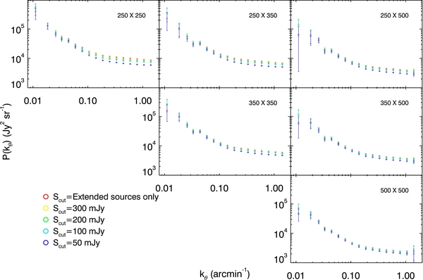
Figure 15. Combined spectra vs. flux cut of masked sources, plotted as circles with error bars. The best estimates of the cirrus spectra in each field (Section 3.3) are removed before combining.
Download figure:
Standard image High-resolution image
Table 8. Best-fit Poisson Levels as Shown in Figure 6
| S > 50 mJy | S > 100 mJy | S > 200 mJy | S > 300 mJy | Extended | |
|---|---|---|---|---|---|
| 250 × 250 | (6.0 ± 0.1) × 103 | (7.4 ± 0.1) × 103 | (8.1 ± 0.1) × 103 | (8.4 ± 0.1) × 103 | (9.0 ± 0.1) × 103 |
| 250 × 350 | (5.1 ± 0.1) × 103 | (6.2 ± 0.1) × 103 | (6.6 ± 0.1) × 103 | (6.7 ± 0.1) × 103 | (7.0 ± 0.1) × 103 |
| 250 × 500 | (3.0 ± 0.0) × 103 | (3.6 ± 0.1) × 103 | (3.8 ± 0.1) × 103 | (3.9 ± 0.1) × 103 | (4.0 ± 0.1) × 103 |
| 350 × 350 | (5.2 ± 0.0) × 103 | (5.9 ± 0.1) × 103 | (6.1 ± 0.1) × 103 | (6.1 ± 0.1) × 103 | (6.2 ± 0.1) × 103 |
| 350 × 500 | (3.1 ± 0.0) × 103 | (3.6 ± 0.0) × 103 | (3.7 ± 0.0) × 103 | (3.7 ± 0.0) × 103 | (3.8 ± 0.0) × 103 |
| 500 × 500 | (2.2 ± 0.0) × 103 | (2.4 ± 0.0) × 103 | (2.4 ± 0.0) × 103 | (2.4 ± 0.0) × 103 | (2.4 ± 0.0) × 103 |
Download table as: ASCIITypeset image
Table 9. Best-fit Poisson Levels for the Alternative Masking Scheme Described in Appendix D.
| S > 50 mJy | S > 100 mJy | S > 200 mJy | S > 300 mJy | Extended | |
|---|---|---|---|---|---|
| 250 × 250 | (5.8 ± 0.1) × 103 | (7.3 ± 0.1) × 103 | (7.9 ± 0.1) × 103 | (8.2 ± 0.1) × 103 | (8.6 ± 0.2) × 103 |
| 250 × 350 | (5.0 ± 0.1) × 103 | (6.0 ± 0.1) × 103 | (6.4 ± 0.1) × 103 | (6.5 ± 0.1) × 103 | (6.7 ± 0.1) × 103 |
| 250 × 500 | (2.9 ± 0.1) × 103 | (3.5 ± 0.1) × 103 | (3.6 ± 0.1) × 103 | (3.7 ± 0.1) × 103 | (3.8 ± 0.1) × 103 |
| 350 × 350 | (4.7 ± 0.1) × 103 | (5.5 ± 0.1) × 103 | (5.7 ± 0.1) × 103 | (5.8 ± 0.1) × 103 | (5.9 ± 0.1) × 103 |
| 350 × 500 | (2.9 ± 0.1) × 103 | (3.4 ± 0.1) × 103 | (3.5 ± 0.1) × 103 | (3.5 ± 0.1) × 103 | (3.5 ± 0.1) × 103 |
| 500 × 500 | (1.9 ± 0.1) × 103 | (2.2 ± 0.1) × 103 | (2.3 ± 0.1) × 103 | (2.3 ± 0.1) × 103 | (2.3 ± 0.1) × 103 |
Download table as: ASCIITypeset image
Table 10. Combined Power Spectra for All Levels of Masking
| kθ | Only Extended Sources Masked | |||||
|---|---|---|---|---|---|---|
| (arcmin−1) | 250 × 250 | 250 × 350 | 250 × 500 | 350 × 350 | 350 × 500 | 500 × 500 |
| 0.011 | (5.15 ± 3.02) × 105 | (3.59 ± 2.45) × 105 | (1.46 ± 1.08) × 105 | (2.70 ± 1.69) × 105 | (1.19 ± 0.76) × 105 | (7.41 ± 3.87) × 104 |
| 0.019 | (1.34 ± 0.43) × 105 | (1.09 ± 0.73) × 105 | (6.28 ± 4.37) × 104 | (1.04 ± 0.42) × 105 | (6.31 ± 3.18) × 104 | (4.45 ± 1.51) × 104 |
| 0.026 | (7.72 ± 1.70) × 104 | (5.80 ± 1.57) × 104 | (4.27 ± 1.08) × 104 | (5.60 ± 1.07) × 104 | (3.62 ± 0.86) × 104 | (2.55 ± 0.46) × 104 |
| 0.033 | (5.18 ± 0.94) × 104 | (3.39 ± 0.67) × 104 | (1.96 ± 0.46) × 104 | (3.27 ± 0.53) × 104 | (1.87 ± 0.37) × 104 | (1.49 ± 0.22) × 104 |
| 0.044 | (4.40 ± 0.54) × 104 | (3.55 ± 0.46) × 104 | (1.95 ± 0.28) × 104 | (3.34 ± 0.37) × 104 | (1.85 ± 0.23) × 104 | (1.23 ± 0.15) × 104 |
| 0.059 | (2.84 ± 0.32) × 104 | (2.27 ± 0.26) × 104 | (1.30 ± 0.17) × 104 | (2.12 ± 0.22) × 104 | (1.26 ± 0.14) × 104 | (8.48 ± 0.95) × 103 |
| 0.079 | (2.27 ± 0.20) × 104 | (1.78 ± 0.14) × 104 | (9.98 ± 0.86) × 103 | (1.61 ± 0.12) × 104 | (9.54 ± 0.74) × 103 | (6.36 ± 0.52) × 103 |
| 0.105 | (1.67 ± 0.11) × 104 | (1.35 ± 0.08) × 104 | (7.60 ± 0.44) × 103 | (1.23 ± 0.06) × 104 | (7.35 ± 0.38) × 103 | (4.79 ± 0.27) × 103 |
| 0.141 | (1.45 ± 0.08) × 104 | (1.16 ± 0.05) × 104 | (6.47 ± 0.31) × 103 | (1.03 ± 0.04) × 104 | (6.15 ± 0.26) × 103 | (3.95 ± 0.19) × 103 |
| 0.187 | (1.23 ± 0.06) × 104 | (9.90 ± 0.42) × 103 | (5.48 ± 0.23) × 103 | (8.79 ± 0.32) × 103 | (5.26 ± 0.18) × 103 | (3.37 ± 0.13) × 103 |
| 0.250 | (1.13 ± 0.05) × 104 | (9.10 ± 0.36) × 103 | (5.08 ± 0.20) × 103 | (8.09 ± 0.27) × 103 | (4.88 ± 0.15) × 103 | (3.15 ± 0.11) × 103 |
| 0.333 | (1.08 ± 0.05) × 104 | (8.61 ± 0.33) × 103 | (4.74 ± 0.17) × 103 | (7.58 ± 0.24) × 103 | (4.53 ± 0.13) × 103 | (2.90 ± 0.09) × 103 |
| 0.445 | (1.03 ± 0.04) × 104 | (8.09 ± 0.28) × 103 | (4.44 ± 0.16) × 103 | (7.05 ± 0.21) × 103 | (4.20 ± 0.12) × 103 | (2.68 ± 0.09) × 103 |
| 0.593 | (9.93 ± 0.39) × 103 | (7.77 ± 0.26) × 103 | (4.29 ± 0.16) × 103 | (6.72 ± 0.20) × 103 | (4.03 ± 0.11) × 103 | (2.58 ± 0.10) × 103 |
| 0.790 | (9.40 ± 0.35) × 103 | (7.38 ± 0.23) × 103 | (4.03 ± 0.17) × 103 | (6.42 ± 0.18) × 103 | (3.81 ± 0.12) × 103 | (2.43 ± 0.13) × 103 |
| 1.054 | (8.92 ± 0.32) × 103 | (7.01 ± 0.22) × 103 | (3.80 ± 0.25) × 103 | (6.12 ± 0.18) × 103 | (3.62 ± 0.18) × 103 | (2.33 ± 0.34) × 103 |
| 1.406 | (8.54 ± 0.31) × 103 | (6.71 ± 0.23) × 103 | (3.59 ± 0.86) × 103 | (5.84 ± 0.24) × 103 | (3.39 ± 0.70) × 103 | (2.50 ± 1.79) × 103 |
| kθ | Sources with S > 300 mJy Masked | |||||
| (arcmin−1) | 250 × 250 | 250 × 350 | 250 × 500 | 350 × 350 | 350 × 500 | 500 × 500 |
| 0.011 | (5.09 ± 2.99) × 105 | (3.57 ± 2.44) × 105 | (1.45 ± 1.09) × 105 | (2.70 ± 1.69) × 105 | (1.19 ± 0.76) × 105 | (7.41 ± 3.88) × 104 |
| 0.019 | (1.34 ± 0.43) × 105 | (1.09 ± 0.74) × 105 | (6.36 ± 4.41) × 104 | (1.04 ± 0.43) × 105 | (6.35 ± 3.19) × 104 | (4.46 ± 1.51) × 104 |
| 0.026 | (7.73 ± 1.70) × 104 | (5.83 ± 1.59) × 104 | (4.31 ± 1.09) × 104 | (5.59 ± 1.07) × 104 | (3.63 ± 0.86) × 104 | (2.56 ± 0.46) × 104 |
| 0.033 | (5.11 ± 0.93) × 104 | (3.39 ± 0.67) × 104 | (1.95 ± 0.45) × 104 | (3.29 ± 0.53) × 104 | (1.88 ± 0.37) × 104 | (1.49 ± 0.22) × 104 |
| 0.044 | (4.32 ± 0.52) × 104 | (3.51 ± 0.46) × 104 | (1.94 ± 0.28) × 104 | (3.32 ± 0.38) × 104 | (1.85 ± 0.23) × 104 | (1.23 ± 0.14) × 104 |
| 0.059 | (2.71 ± 0.30) × 104 | (2.20 ± 0.26) × 104 | (1.26 ± 0.16) × 104 | (2.11 ± 0.23) × 104 | (1.25 ± 0.14) × 104 | (8.42 ± 0.94) × 103 |
| 0.079 | (2.17 ± 0.17) × 104 | (1.73 ± 0.13) × 104 | (9.77 ± 0.84) × 103 | (1.60 ± 0.12) × 104 | (9.46 ± 0.73) × 103 | (6.31 ± 0.51) × 103 |
| 0.105 | (1.57 ± 0.08) × 104 | (1.30 ± 0.07) × 104 | (7.42 ± 0.43) × 103 | (1.22 ± 0.06) × 104 | (7.31 ± 0.39) × 103 | (4.77 ± 0.28) × 103 |
| 0.141 | (1.36 ± 0.06) × 104 | (1.11 ± 0.04) × 104 | (6.30 ± 0.28) × 103 | (1.02 ± 0.04) × 104 | (6.10 ± 0.25) × 103 | (3.93 ± 0.18) × 103 |
| 0.187 | (1.15 ± 0.04) × 104 | (9.48 ± 0.31) × 103 | (5.33 ± 0.20) × 103 | (8.68 ± 0.26) × 103 | (5.21 ± 0.17) × 103 | (3.35 ± 0.13) × 103 |
| 0.250 | (1.06 ± 0.04) × 104 | (8.71 ± 0.27) × 103 | (4.92 ± 0.17) × 103 | (8.00 ± 0.22) × 103 | (4.84 ± 0.14) × 103 | (3.13 ± 0.11) × 103 |
| 0.333 | (1.00 ± 0.04) × 104 | (8.19 ± 0.24) × 103 | (4.58 ± 0.14) × 103 | (7.49 ± 0.19) × 103 | (4.49 ± 0.12) × 103 | (2.88 ± 0.09) × 103 |
| 0.445 | (9.53 ± 0.32) × 103 | (7.69 ± 0.21) × 103 | (4.29 ± 0.13) × 103 | (6.96 ± 0.17) × 103 | (4.16 ± 0.11) × 103 | (2.66 ± 0.09) × 103 |
| 0.593 | (9.22 ± 0.31) × 103 | (7.39 ± 0.20) × 103 | (4.14 ± 0.13) × 103 | (6.64 ± 0.16) × 103 | (3.99 ± 0.11) × 103 | (2.56 ± 0.10) × 103 |
| 0.790 | (8.81 ± 0.29) × 103 | (7.05 ± 0.19) × 103 | (3.91 ± 0.14) × 103 | (6.35 ± 0.15) × 103 | (3.78 ± 0.11) × 103 | (2.42 ± 0.13) × 103 |
| 1.054 | (8.42 ± 0.27) × 103 | (6.74 ± 0.18) × 103 | (3.70 ± 0.22) × 103 | (6.06 ± 0.16) × 103 | (3.59 ± 0.17) × 103 | (2.32 ± 0.34) × 103 |
| 1.406 | (8.15 ± 0.27) × 103 | (6.50 ± 0.20) × 103 | (3.51 ± 0.75) × 103 | (5.80 ± 0.22) × 103 | (3.37 ± 0.67) × 103 | (2.49 ± 1.78) × 103 |
| kθ | Sources with S > 200 mJy Masked | |||||
| (arcmin−1) | 250 × 250 | 250 × 350 | 250 × 500 | 350 × 350 | 350 × 500 | 500 × 500 |
| 0.011 | (5.05 ± 2.96) × 105 | (3.55 ± 2.43) × 105 | (1.44 ± 1.08) × 105 | (2.70 ± 1.68) × 105 | (1.19 ± 0.77) × 105 | (7.41 ± 3.88) × 104 |
| 0.019 | (1.34 ± 0.43) × 105 | (1.09 ± 0.74) × 105 | (6.42 ± 4.42) × 104 | (1.05 ± 0.43) × 105 | (6.36 ± 3.20) × 104 | (4.46 ± 1.51) × 104 |
| 0.026 | (7.69 ± 1.69) × 104 | (5.76 ± 1.57) × 104 | (4.32 ± 1.09) × 104 | (5.62 ± 1.07) × 104 | (3.63 ± 0.86) × 104 | (2.56 ± 0.46) × 104 |
| 0.033 | (5.05 ± 0.92) × 104 | (3.34 ± 0.66) × 104 | (1.91 ± 0.45) × 104 | (3.26 ± 0.52) × 104 | (1.87 ± 0.36) × 104 | (1.49 ± 0.22) × 104 |
| 0.044 | (4.26 ± 0.52) × 104 | (3.48 ± 0.45) × 104 | (1.93 ± 0.27) × 104 | (3.31 ± 0.37) × 104 | (1.84 ± 0.23) × 104 | (1.23 ± 0.14) × 104 |
| 0.059 | (2.70 ± 0.30) × 104 | (2.19 ± 0.25) × 104 | (1.26 ± 0.17) × 104 | (2.09 ± 0.22) × 104 | (1.24 ± 0.14) × 104 | (8.42 ± 0.94) × 103 |
| 0.079 | (2.14 ± 0.17) × 104 | (1.71 ± 0.13) × 104 | (9.73 ± 0.85) × 103 | (1.59 ± 0.11) × 104 | (9.42 ± 0.74) × 103 | (6.31 ± 0.52) × 103 |
| 0.105 | (1.54 ± 0.08) × 104 | (1.29 ± 0.06) × 104 | (7.40 ± 0.42) × 103 | (1.21 ± 0.06) × 104 | (7.27 ± 0.39) × 103 | (4.77 ± 0.28) × 103 |
| 0.141 | (1.32 ± 0.05) × 104 | (1.10 ± 0.04) × 104 | (6.23 ± 0.28) × 103 | (1.01 ± 0.04) × 104 | (6.08 ± 0.25) × 103 | (3.93 ± 0.18) × 103 |
| 0.187 | (1.11 ± 0.04) × 104 | (9.30 ± 0.29) × 103 | (5.26 ± 0.19) × 103 | (8.60 ± 0.26) × 103 | (5.19 ± 0.17) × 103 | (3.35 ± 0.13) × 103 |
| 0.250 | (1.02 ± 0.03) × 104 | (8.54 ± 0.24) × 103 | (4.87 ± 0.16) × 103 | (7.92 ± 0.21) × 103 | (4.81 ± 0.14) × 103 | (3.13 ± 0.11) × 103 |
| 0.333 | (9.58 ± 0.30) × 103 | (7.99 ± 0.21) × 103 | (4.52 ± 0.13) × 103 | (7.41 ± 0.18) × 103 | (4.46 ± 0.12) × 103 | (2.88 ± 0.09) × 103 |
| 0.445 | (9.12 ± 0.28) × 103 | (7.51 ± 0.19) × 103 | (4.23 ± 0.12) × 103 | (6.88 ± 0.16) × 103 | (4.13 ± 0.10) × 103 | (2.66 ± 0.09) × 103 |
| 0.593 | (8.85 ± 0.27) × 103 | (7.22 ± 0.18) × 103 | (4.08 ± 0.12) × 103 | (6.57 ± 0.16) × 103 | (3.96 ± 0.10) × 103 | (2.56 ± 0.10) × 103 |
| 0.790 | (8.46 ± 0.25) × 103 | (6.90 ± 0.17) × 103 | (3.85 ± 0.13) × 103 | (6.30 ± 0.15) × 103 | (3.75 ± 0.11) × 103 | (2.42 ± 0.13) × 103 |
| 1.054 | (8.12 ± 0.24) × 103 | (6.60 ± 0.17) × 103 | (3.65 ± 0.20) × 103 | (6.02 ± 0.15) × 103 | (3.57 ± 0.16) × 103 | (2.32 ± 0.33) × 103 |
| 1.406 | (7.89 ± 0.25) × 103 | (6.37 ± 0.18) × 103 | (3.46 ± 0.71) × 103 | (5.76 ± 0.21) × 103 | (3.36 ± 0.65) × 103 | (2.49 ± 1.77) × 103 |
| kθ | Sources with S > 100 mJy Masked | |||||
| (arcmin−1) | 250 × 250 | 250 × 350 | 250 × 500 | 350 × 350 | 350 × 500 | 500 × 500 |
| 0.011 | (4.88 ± 2.91) × 105 | (3.44 ± 2.40) × 105 | (1.37 ± 1.06) × 105 | (2.65 ± 1.67) × 105 | (1.17 ± 0.76) × 105 | (7.41 ± 3.88) × 104 |
| 0.019 | (1.33 ± 0.43) × 105 | (1.07 ± 0.73) × 105 | (6.31 ± 4.39) × 104 | (1.04 ± 0.42) × 105 | (6.37 ± 3.20) × 104 | (4.45 ± 1.51) × 104 |
| 0.026 | (7.34 ± 1.63) × 104 | (5.53 ± 1.53) × 104 | (4.31 ± 1.09) × 104 | (5.46 ± 1.05) × 104 | (3.60 ± 0.85) × 104 | (2.55 ± 0.46) × 104 |
| 0.033 | (4.83 ± 0.89) × 104 | (3.23 ± 0.65) × 104 | (1.87 ± 0.44) × 104 | (3.20 ± 0.51) × 104 | (1.82 ± 0.36) × 104 | (1.47 ± 0.22) × 104 |
| 0.044 | (4.20 ± 0.51) × 104 | (3.43 ± 0.45) × 104 | (1.91 ± 0.27) × 104 | (3.28 ± 0.37) × 104 | (1.83 ± 0.23) × 104 | (1.22 ± 0.14) × 104 |
| 0.059 | (2.63 ± 0.29) × 104 | (2.15 ± 0.25) × 104 | (1.24 ± 0.16) × 104 | (2.06 ± 0.22) × 104 | (1.23 ± 0.14) × 104 | (8.36 ± 0.94) × 103 |
| 0.079 | (2.04 ± 0.17) × 104 | (1.67 ± 0.13) × 104 | (9.54 ± 0.84) × 103 | (1.57 ± 0.12) × 104 | (9.36 ± 0.74) × 103 | (6.28 ± 0.51) × 103 |
| 0.105 | (1.46 ± 0.07) × 104 | (1.25 ± 0.06) × 104 | (7.25 ± 0.41) × 103 | (1.19 ± 0.06) × 104 | (7.20 ± 0.38) × 103 | (4.74 ± 0.27) × 103 |
| 0.141 | (1.23 ± 0.04) × 104 | (1.05 ± 0.04) × 104 | (6.04 ± 0.27) × 103 | (9.84 ± 0.37) × 103 | (5.99 ± 0.25) × 103 | (3.92 ± 0.18) × 103 |
| 0.187 | (1.03 ± 0.03) × 104 | (8.84 ± 0.26) × 103 | (5.10 ± 0.18) × 103 | (8.35 ± 0.24) × 103 | (5.08 ± 0.16) × 103 | (3.32 ± 0.12) × 103 |
| 0.250 | (9.39 ± 0.27) × 103 | (8.08 ± 0.21) × 103 | (4.69 ± 0.14) × 103 | (7.68 ± 0.19) × 103 | (4.71 ± 0.13) × 103 | (3.11 ± 0.10) × 103 |
| 0.333 | (8.79 ± 0.24) × 103 | (7.52 ± 0.18) × 103 | (4.34 ± 0.12) × 103 | (7.14 ± 0.17) × 103 | (4.35 ± 0.11) × 103 | (2.85 ± 0.09) × 103 |
| 0.445 | (8.33 ± 0.22) × 103 | (7.05 ± 0.16) × 103 | (4.05 ± 0.11) × 103 | (6.65 ± 0.15) × 103 | (4.03 ± 0.10) × 103 | (2.64 ± 0.08) × 103 |
| 0.593 | (8.09 ± 0.22) × 103 | (6.78 ± 0.16) × 103 | (3.91 ± 0.11) × 103 | (6.37 ± 0.14) × 103 | (3.87 ± 0.10) × 103 | (2.55 ± 0.09) × 103 |
| 0.790 | (7.74 ± 0.21) × 103 | (6.49 ± 0.15) × 103 | (3.69 ± 0.12) × 103 | (6.11 ± 0.14) × 103 | (3.68 ± 0.10) × 103 | (2.40 ± 0.13) × 103 |
| 1.054 | (7.49 ± 0.20) × 103 | (6.23 ± 0.14) × 103 | (3.50 ± 0.19) × 103 | (5.86 ± 0.14) × 103 | (3.51 ± 0.16) × 103 | (2.31 ± 0.33) × 103 |
| 1.406 | (7.31 ± 0.21) × 103 | (6.03 ± 0.16) × 103 | (3.31 ± 0.67) × 103 | (5.64 ± 0.20) × 103 | (3.30 ± 0.63) × 103 | (2.48 ± 1.75) × 103 |
| kθ | Sources with S > 50 mJy Masked | |||||
| (arcmin−1) | 250 × 250 | 250 × 350 | 250 × 500 | 350 × 350 | 350 × 500 | 500 × 500 |
| 0.011 | (4.00 ± 2.62) × 105 | (2.55 ± 2.08) × 105 | (1.09 ± 0.95) × 105 | (2.00 ± 1.44) × 105 | (9.52 ± 6.76) × 104 | (6.80 ± 3.64) × 104 |
| 0.019 | (1.25 ± 0.41) × 105 | (9.88 ± 6.98) × 104 | (5.88 ± 4.26) × 104 | (9.39 ± 3.96) × 104 | (5.90 ± 3.03) × 104 | (4.22 ± 1.45) × 104 |
| 0.026 | (6.64 ± 1.50) × 104 | (4.80 ± 1.36) × 104 | (4.17 ± 1.05) × 104 | (4.94 ± 0.96) × 104 | (3.43 ± 0.81) × 104 | (2.54 ± 0.46) × 104 |
| 0.033 | (4.46 ± 0.83) × 104 | (2.87 ± 0.58) × 104 | (1.72 ± 0.40) × 104 | (2.89 ± 0.47) × 104 | (1.64 ± 0.33) × 104 | (1.38 ± 0.21) × 104 |
| 0.044 | (3.78 ± 0.46) × 104 | (3.08 ± 0.41) × 104 | (1.75 ± 0.25) × 104 | (2.96 ± 0.34) × 104 | (1.68 ± 0.21) × 104 | (1.17 ± 0.14) × 104 |
| 0.059 | (2.38 ± 0.27) × 104 | (1.95 ± 0.23) × 104 | (1.15 ± 0.15) × 104 | (1.88 ± 0.20) × 104 | (1.13 ± 0.13) × 104 | (7.91 ± 0.90) × 103 |
| 0.079 | (1.77 ± 0.14) × 104 | (1.47 ± 0.12) × 104 | (8.62 ± 0.77) × 103 | (1.43 ± 0.10) × 104 | (8.57 ± 0.68) × 103 | (5.97 ± 0.49) × 103 |
| 0.105 | (1.28 ± 0.07) × 104 | (1.10 ± 0.06) × 104 | (6.50 ± 0.38) × 103 | (1.07 ± 0.05) × 104 | (6.50 ± 0.34) × 103 | (4.43 ± 0.26) × 103 |
| 0.141 | (1.03 ± 0.04) × 104 | (8.85 ± 0.33) × 103 | (5.30 ± 0.23) × 103 | (8.59 ± 0.32) × 103 | (5.31 ± 0.21) × 103 | (3.65 ± 0.16) × 103 |
| 0.187 | (8.57 ± 0.26) × 103 | (7.48 ± 0.21) × 103 | (4.44 ± 0.15) × 103 | (7.40 ± 0.21) × 103 | (4.53 ± 0.14) × 103 | (3.11 ± 0.11) × 103 |
| 0.250 | (7.76 ± 0.22) × 103 | (6.79 ± 0.17) × 103 | (4.05 ± 0.12) × 103 | (6.73 ± 0.17) × 103 | (4.14 ± 0.11) × 103 | (2.88 ± 0.09) × 103 |
| 0.333 | (7.23 ± 0.18) × 103 | (6.25 ± 0.14) × 103 | (3.69 ± 0.10) × 103 | (6.24 ± 0.14) × 103 | (3.77 ± 0.09) × 103 | (2.63 ± 0.08) × 103 |
| 0.445 | (6.76 ± 0.17) × 103 | (5.79 ± 0.13) × 103 | (3.41 ± 0.09) × 103 | (5.80 ± 0.12) × 103 | (3.49 ± 0.08) × 103 | (2.44 ± 0.07) × 103 |
| 0.593 | (6.47 ± 0.16) × 103 | (5.50 ± 0.12) × 103 | (3.25 ± 0.09) × 103 | (5.50 ± 0.12) × 103 | (3.32 ± 0.08) × 103 | (2.36 ± 0.08) × 103 |
| 0.790 | (6.18 ± 0.15) × 103 | (5.25 ± 0.11) × 103 | (3.09 ± 0.10) × 103 | (5.31 ± 0.11) × 103 | (3.19 ± 0.08) × 103 | (2.27 ± 0.11) × 103 |
| 1.054 | (6.00 ± 0.15) × 103 | (5.08 ± 0.11) × 103 | (2.94 ± 0.15) × 103 | (5.18 ± 0.12) × 103 | (3.09 ± 0.13) × 103 | (2.20 ± 0.29) × 103 |
| 1.406 | (5.93 ± 0.16) × 103 | (5.00 ± 0.13) × 103 | (2.80 ± 0.53) × 103 | (5.05 ± 0.17) × 103 | (2.96 ± 0.53) × 103 | (2.37 ± 1.57) × 103 |
Note. At each wavelength, only sources above the flux cut are masked.
APPENDIX E:
Poisson levels for the default masking scheme (in which masked sources are identified uniquely for each band) are tabulated in Table 8, while Poisson levels for the alternate masking scheme (in which masked sources in all bands are those identified at 250 μm) are tabulated in Table 9. The cirrus-subtracted, combined power spectra and 1σ errors for all masking levels (as shown in Figure 5) are tabulated in Table 10.
Footnotes
- *
Herschel is an ESA space observatory with science instruments provided by European-led Principal Investigator consortia and with important participation from NASA.
- 34
- 35
- 36
- 37
- 38
- 39
- 40
The gd are in fact the deviations from 1.0 of the detector gains already applied by HIPE.
- 41
- 42
Tabulations of the Neptune and Uranus brightness temperatures are available from the ESA Herschel Science Centre ftp://ftp.sciops.esa.int/pub/hsc-calibration
- 43