


ABSTRACT
Recent combined observations from the first three years of Interstellar Boundary Explorer (IBEX) data allow us to examine the heliosphere's downwind region—the heliotail—for the first time. In contrast to a preliminary identification of a narrow "offset heliotail" structure, we find a broad slow solar wind plasma sheet crossing essentially the entire downwind side of the heliosphere at low to mid-latitudes, with fast wind tail regions to the north and south. The slow wind plasma sheet exhibits the steepest ENA spectra in the IBEX sky maps, appears as a two-lobed structure (lobes on the port and starboard sides), and is twisted in the sense of (but at a smaller angle than) the external magnetic field. The overall heliotail structure clearly demonstrates the intermediate nature of the heliosphere's interstellar interaction, where both the external dynamic and magnetic pressures strongly affect the heliosphere.
Export citation and abstract BibTeX RIS
1. INTRODUCTION
The Interstellar Boundary Explorer (IBEX; McComas et al. 2009a) is the first mission dedicated to imaging the heliosphere's global interaction with the interstellar medium. IBEX does this by making energy-resolved all-sky maps of energetic neutral atoms (ENAs) over the energy range from ∼0.1 to 6 keV. The first IBEX sky maps showed a "globally distributed flux" of smoothly varying ENA emissions from all directions and discovered a completely unexpected "ribbon" of two to three times enhanced ENA emissions (McComas et al. 2009b). The ribbon comprises a narrow (∼20° wide) arc of enhanced ENA emissions forming a nearly complete circle (∼300°) apparently centered on the most likely direction of the interstellar magnetic field outside the heliosphere (McComas et al. 2009b; Fuselier et al. 2009; Funsten et al. 2009b; Schwadron et al. 2009a). Since the original articles in Science, there have been numerous studies and papers on various aspects of the IBEX observations; McComas et al. (2011b) provides a brief recent review.
Another important advancement in our understanding of the interaction is that there is almost certainly no bow shock ahead of the heliosphere in the interstellar medium (McComas et al. 2012a). This result was based on the combination of (1) new IBEX observations of the interstellar flow that indicates a slower relative motion (and an inflow direction of (79°, −5°) in ecliptic J2000 longitude and latitude; Bzowski et al. 2012; Möbius et al. 2012; McComas et al. 2012a); and (2) multiple lines of evidence that the interstellar magnetic field is relatively strong (⩾3 μG). Such a large magnetic field strength is indicated by the significant asymmetry of the Voyager 1 and 2 termination shock crossings (Stone et al. 2008), which requires an asymmetric pressure that is likely caused by a strong external magnetic field (Opher et al. 2006; Washimi et al. 2007). In addition, some simulations infer high field values (e.g., Ratkiewicz & Grygorczuk (2008) found ∼3.8 μG). Schwadron et al. (2011) used a fitting technique to separate the globally distributed ENA fluxes from the ribbon for the first year of IBEX observations. That study indicated a magnetic field strength of ∼3.3 μG from pressure balance arguments. Finally, Zank et al. (2013) used MHD simulations to show that Lyα observations of the hydrogen wall are quite consistent with an ∼3 μG external field and no bow shock.
Together, the discovery of the IBEX ribbon and the weaker bow-shock-less interaction strongly support the notion that the heliosphere's current interstellar interaction is truly intermediate between Parker's (1961) extreme's of the possible interaction, with comparable dynamic and magnetic pressures governing the interaction, as suggested by McComas et al. (2009b)—see Figure 1. For the likely configuration with the local interstellar magnetic field significantly inclined (∼45°) from the inflow (or upwind) direction, such an interaction begs the question of the shape and structure of the heliosphere generally, and the existence and configuration of a heliotail specifically.
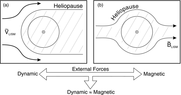
Figure 1. Extremes of the heliospheric interaction described by Parker (1961). Our heliosphere lies squarely between them with the external dynamic and magnetic pressures having comparable effects on the heliosphere. Figure taken from McComas et al. (2009b).
Download figure:
Standard image High-resolution imageA major discovery of Schwadron et al. (2011) was a clearly identifiable structure in the globally distributed flux that is offset from the downwind (anti-ram) interstellar flow direction. This structure appeared to be centered between the downwind direction and the downfield direction of the external magnetic field, and has been referred to as the "offset heliotail." Note that we use the directions inferred from the center of the ribbon (Funsten et al. 2009b) to define the interstellar "upfield" (λ, β) = (−139°, 39°) ecliptic (J2000) and "downfield" (41°, −39°) viewing directions as the external magnetic field direction on the same side as the upwind (−101°, 5°) and downwind (79°, −5°) viewing directions, respectively.
Most recently, McComas et al. (2012b) provided complete and validated observations from the first three years (2009–2011) of IBEX ENA observations. These authors also corrected the ENA observations for both the time-variable cosmic ray background and for orbit-by-orbit variations in the survival probability for ENAs reaching 1 AU from the outer heliosphere. McComas et al. (2012b) also quantified an overall reduction in ENA emissions over the three years of IBEX observations (2009–2011); the ribbon flux has decreased by the largest fraction, with no flux reduction (and possibly an increase) from the offset heliotail direction. The energy spectral index γ for this region, and more broadly across the downwind part of the sky, is larger than for other directions and ranges typically from γ ∼ 2–3.
A variety of models have been used to explore the possible processes responsible for ENA emissions from the heliotail region. Some of these have shown a structured plasma in the heliotail region (e.g., Izmodenov et al. 2009; Zank et al. 2009 and references therein) that may vary over the solar cycle (e.g., Sternall et al. 2008). To the best of our knowledge, however, no models have shown a strongly offset heliotail (tens of degrees from the downwind direction), with the possible exception of the model of Prested (Prested et al. 2008; Schwadron et al. 2009b).
In this study, we use the combined 2009–2011 IBEX data set validated by McComas et al. (2012b) to examine the heliotail in detail for the first time. We also discuss the observed heliotail's implications for the heliosphere's global interstellar interaction.
2. OBSERVATIONS
We examine the first three years of IBEX ENA observations including extinction (ENA losses en route in from the outer heliosphere) and Compton–Getting (C–G) corrections (McComas et al. 2012b) from the IBEX-Hi instrument (Funsten et al. 2009a). Figure 2 shows ENA sky maps centered on (21°, −6°) ecliptic longitude and latitude—the approximate direction of the offset heliotail identified by Schwadron et al. (2011). From this viewing perspective, it is easy to see that this region has a different energy spectrum than most of the sky, with an enhancement of low energy ENAs and dearth of high energy ones.
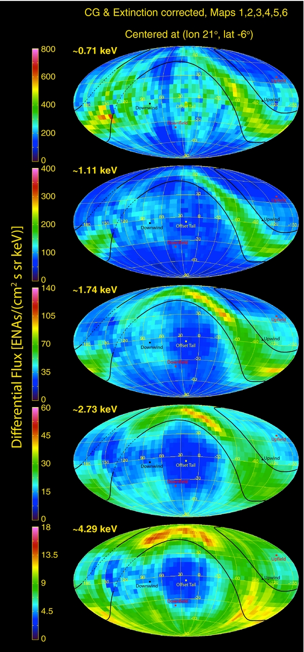
Figure 2. ENA fluxes for five energy passbands (central energies listed) covering a combined energy range from ∼0.5 to 6 keV FWHM. The plots are Mollweide projections as viewed from the inside looking out, and approximately centered on the offset heliotail direction as indicated by the lowest fluxes at high energies; the approximate ribbon boundaries are indicated by black lines.
Download figure:
Standard image High-resolution imageThe Schwadron et al. (2011) study only had the first year of IBEX observations to work with and the statistics were limited. In that study, the offset heliotail seemed to be in a direction intermediate between the downwind (black dot in Figure 2) and interstellar downfield (red dot) directions. However, with enhanced statistics from three years of observations (and improved culling and correction factors), rather than being intermediate in direction between the downwind and downfield directions, this structure appears to be shifted primarily in ecliptic longitude (even beyond the downfield direction), with only a small shift in ecliptic latitude toward the downfield direction.
In order to determine the center of this offset heliotail, we plot in Figure 3 the highest three energy channels (columns) of the three year combined data, as above, for a limited region (top row) and their smoothed fits (bottom row). The smoothing was performed by applying a third degree surface polynomial fitting to the ENA fluxes. The locations of the lowest flux values from the fits are indicated by the white numbers for each energy band. With 3° smoothing pixels, these lowest values are at ecliptic longitudes and latitudes of 1.7 keV (33°, −3°), 2.7 keV (21°, −9), and 4.3 keV (9°, −9). This indicates a consistent progression of the center of the structure direction, and therefore the structure itself, toward the downwind direction (larger ecliptic longitudes and less negative heliolatitudes) for higher energy ENAs. The total change for the centers of the 1.7–4.3 keV channels is +24° in ecliptic longitude and +6° in ecliptic latitude.

Figure 3. ENA fluxes (top row) and smoothed fluxes (bottom) for 1.7, 2.7, and 4.3 keV central energies (columns), shown in ecliptic coordinates. The minimum values (white numbers indicating the respective energy bands) show a clear progression with the center of the structure being closer to the downwind direction with increasing energy, as indicated by the arrow pointing toward the downwind direction (79°, −5°).
Download figure:
Standard image High-resolution imageFigure 4 quantifies the energy spectral index over the sky, using the five energy bands shown in Figure 2. The tail appears as the steepest slope region in the map, with the slopes being generally steeper at low latitudes and within the ribbon (McComas et al. 2009b). While a single spectral slope is generally a good fit for low to mid latitudes, the highest latitude pixels typically show a spectral break and are much better fit by two components (Dayeh et al. 2011, 2012) not shown here; still, high latitude spectra (especially outside the ribbon) are significantly less steep than low latitude ones.
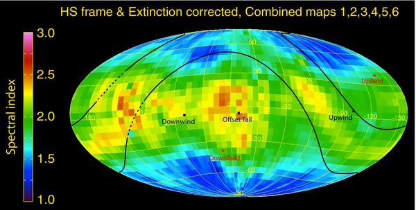
Figure 4. Spectral slope plot centered on the offset heliotail direction as in Figure 2.
Download figure:
Standard image High-resolution imageInterestingly, another similarly steep spectral structure appears to the left of the offset tail in Figure 4, on the other side of the downwind direction and at least partially within the black lines that generally represent the ribbon region; we dashed the lines through this region as the ribbon is uncertain here. In order to assess this structure, in the top panel of Figure 5, we replot the spectral slopes in a new Mollweide projection that is centered directly on the downwind direction. This projection suggests that the heliotail might actually be a much larger structure, spanning essentially the entire downwind half of the sky, and including two "lobes"—a port lobe that was previously identified as the offset heliotail, and a starboard lobe of similar, but somewhat smaller, size. (Note that we use nautical port and starboard designations to identify the sides of the heliosphere as it moves (like a vessel) through the interstellar medium. This nomenclature removes the ambiguity of which direction one is looking; for example, Figure 5 is the view from inside looking outward and centered on the downwind direction, so port is on the right.) The broad, two lobed tail structure (1) is roughly (although not precisely) centered on the downwind direction, (2) appears narrower in height (latitude) near the middle, and (3) is slightly tilted (∼10°) in the sense (but only a fraction of the angle) of the external field orientation. In order to further validate these results and ensure that they were not driven by any (small) residual noise in the lowest energy channel, we redid the same analysis using only the four highest energies and found extremely similar results.

Figure 5. The top is the same as Figure 4, but centered on the downwind direction; a common color bar is used in both figures. The bottom panel shows a fourth order polynomial smoothing for the region indicated. Note the appearance of a two-lobed structure in the spectral slope map, which is roughly centered on the downwind direction and appears to be slightly tilted toward the direction of the external field. Here we observationally define four regions of the tailward side of the heliosphere (inside the terminator indicated by black circle)—the north and south regions of very low spectral slope and the port and starboard lobes of the low/mid latitude region of high spectral slope.
Download figure:
Standard image High-resolution imageFor completeness, Figure 6 shows the five individual flux maps as in Figure 2, but centered on the downwind direction. While not as easy to see as in the spectral index maps, a two lobed structure is apparent at least in the lowest and couple highest energy steps.

Figure 6. Same as Figure 2, but centered on the downwind direction; a common color bar is used in both figures.
Download figure:
Standard image High-resolution imageThe starboard tail lobe poses a particularly difficult observational issue for IBEX as this region is the most poorly sampled and has the poorest statistics anywhere in the IBEX sky maps. This is because of how IBEX data is taken (measuring ENAs from great circles roughly perpendicular to the spacecraft's Sun-pointed spin axis; see McComas et al. 2009a and references therein) and the fact that the ENA "bright" magnetosphere therefore always occults viewing from the same portion of the sky (Schwadron et al. 2009b). This is why the starboard lobe was not previously found and required the full first three years of observations and statistics to identify and examine. We note that in the process of putting IBEX into a long term stable lunar synchronous orbit (McComas et al. 2011a), we also adjusted the orbital parameters such that the orbit rotates and moves the location of the magnetospheric hole. Thus, much better statistics from this critical region will be made over the next several years of IBEX's extended mission.
In order to assess if the starboard lobe appears to be centered at different locations for different energies, as the port lobe does, we redo the analysis from Figure 3. Figure 7 shows this analysis for the starboard lobe, and again, the center of the lobe appears to move toward the downwind direction at increasingly higher energies. For the starboard lobe, the motion from pass bands centered at 1.7–4.3 keV moves a net angle of (−24°, −18°) in longitude and latitude, toward the down tail direct. This shifting toward the downwind direction is quantitatively very similar to that for the port lobe but from the opposite side. This common feature strongly suggests that the two lobes are physically similar and related structures and that they both are components of the heliotail.
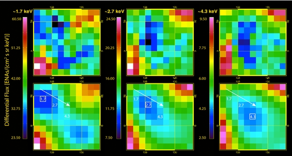
Figure 7. Top three energies like Figure 3, but for starboard side lobe. Again, the structure shows a clear progression toward the downwind direction (arrow) with increasing energy.
Download figure:
Standard image High-resolution image3. DISCUSSION
To summarize the observational features, the heliotail includes a broad low- to mid-latitude structure, which has an excess of lower energy ENAs (<1 keV) and a deficit at higher energies (>2 keV), producing a relatively steep power law energy spectrum (γ = 2–3) compared to the rest of the sky. This structure is large, spanning nearly 180° in longitude, but appears latitudinally thinner in the middle and at the edges in the IBEX ENA observations, and thus, we describe it as having two lobes. The lobes are roughly centered on the downwind direction, and the port lobe appears somewhat larger than the starboard one. Overall, the two-lobe structure is tilted in the sense of the external magnetic fields, but at only a fraction of the angle of that field. Emissions from both lobes are centered closer to the downwind direction with increasing energies across the ENA energy bands centered at 1.7, 2.7, and 4.3 keV.
Unlike the IBEX ribbon, which may well come from ENA emissions beyond the heliopause (e.g., from a "secondary ENA source; McComas et al. 2009b; Heerikhuisen et al. 2010; Chalov et al. 2010; Schwadron & McComas 2013), emissions from the heliotail are almost certainly coming from the region beyond the termination shock, but still inside the heliopause, just as they do for the rest of the globally distributed flux (McComas et al. 2009b; Schwadron et al. 2011). Ecliptic ordering of the heliotail structure clearly indicates the imprint of the solar wind's latitudinal structure in these emissions. The generally steeper power law spectral distributions at low to mid-latitudes compared to higher latitudes is consistent with a solar wind latitudinal structure around solar minimum, with fast, tenuous solar wind from large circumpolar coronal holes at high latitudes and slower and denser solar wind at lower latitudes (McComas 1998; McComas et al. 2008).
Figure 8 shows a highly schematic diagram of the notional heliotail configuration (a) in the noon–midnight meridian and (b) as viewed looking down the tail, compared to (c) the ENA spectral slope observations from Figure 5. In this figure, for solar minimum conditions, faster wind from the high latitude regions largely fills the north and south regions of the tail. In contrast, a broad "slow solar wind plasma sheet" should run longitudinally across the tail, comprising both the port and starboard lobes. Slow wind initially headed in the upwind direction should also fill a thin layer just inside of the heliopause as shown. We note that while the structure in Figure 8 is visually reminiscent of a cut through Earth's magnetotail, the regions and their physical sources are quite different.
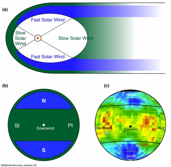
Figure 8. Schematic diagram showing (a) a meridional cut through heliotail, (b) a cut as viewed looking down the tail, and (c) the IBEX spectral index observations from Figure 5 for comparison (note that this is a Mollweide projection spanning the entire tailward hemisphere). Fast solar wind regions in (a) and (b) are indicated in blue and slow solar wind regions in green. The tail structure in (a) is shown fading out with distance as charge exchange losses deplete the heliospheric ions.
Download figure:
Standard image High-resolution imageSolar wind ions in the inner heliosheath are lost through charge exchange—this is actually the signal that IBEX observes. A typical distance to lose 1/e of the slow solar wind ions in the inner heliosheath/tail is ∼120 AU ("cooling distance" from Schwadron et al. 2011); in the fast wind, the comparable distances should be roughly twice as long. This mechanism produces a heliotail where different portions of the tail have different lengths and effectively "evaporates" almost all of the tail ions within ∼1000 AU. Thus, in Figure 8, we also schematically indicate this process by the fading out of the heliospheric tail ions. We note that at greater distances, the tail should "pinch" in as the external magnetic and particle pressures continuous to push in from the sides. Of course, ENAs also continue to re-ionize and re-neutralize over the scales of hundreds of AU, so there should be a broader downwind region of coupled heliospheric and interstellar ions and neutrals in an extended "wake" region behind the heliosphere (not shown).
Comparing the low to mid-latitude ENA emissions at various longitudes, the directions down the tail are the steepest, with the largest fluxes of low energy ENAs and smallest fluxes of high energy ones. We attribute this to the continued slowing of the bulk solar wind heading toward the tail, owing to continued addition of pickup ions. In the upwind direction, it takes typical ∼400 km s−1 slow solar wind about one year to reach the termination shock at ∼100 AU. By this time, the addition of pickup ions has slowed the solar wind flow ∼50 km s−1 to ∼350 km s−1. In the downwind direction, the termination shock is much farther from the Sun (if it even exists as a shock), so the continuing addition of pickup ions further slows the wind, perhaps by as much as another 50–100 km s−1. Once thermalized at the shock (or through other processes), such slower solar wind would naturally produce the steepest energy spectra, as observed by IBEX.
The appearance of lobes of low to mid-latitude emissions instead of a flat emission structure across the tail could be due to geometric effects based on the viewing geometry and line of sight (LOS) integration path lengths for the observed ENAs. Reflecting on the configuration shown in Figure 8, LOSs across the slow wind portion of the inner heliosheath/tail (between the termination shock and heliopause) would be longest in the ecliptic plane. For latitudes further from the ecliptic, these LOSs would be progressively shorter for angles farther from the downwind longitude, toward the sides of the tail. In addition, very close to the downwind longitude LOSs would only have limited extents through the slow wind region and rapidly pierce out into the higher wind portions, where the steep spectral emissions are not produced.
The "folding" of the low to mid-latitude lobes closer to the downwind direction with increasing energy could have several explanations. For example, we cannot rule out time variations since the higher energy ENAs travel faster and represent newer samples of an emission region, compared to lower energy ENAs. On the other hand, the same simple geometric effect that may explain the appearance of lobes can also explain this progression. Higher energy ENAs represent longer LOS integration path lengths owing to both less charge exchange loss for a given distance traveled down tail and less extinction of the ENAs coming back inward. Therefore, the center of emission structures will reflect different integration path lengths with higher energies, naturally representing directions closer to the longest LOSs directly down tail.
Notably missing from this study is the relationship of the heliotail to the most obvious ENA structure in the sky—the IBEX ribbon. Earlier studies suggested that the ribbon marked a nearly complete circle in the sky. The gap in the ribbon observations passes through the magnetospheric viewing hole of significantly lower statistics (dashed portion of the lines in Figures 2 and 4) and so it was hard to determine if the ribbon produced a complete circle. Coincidently, this poorly observed region is also roughly through the starboard side of the downwind region.
We argue here that the spectrally steep structure on this side of the downwind direction region is in fact primarily the starboard slow solar wind lobe of the heliotail with little, if any, superposed ribbon ENAs. This would also be consistent with most of the proposed ribbon generation mechanisms, which produce no or at least far fewer ribbon ENAs toward the downwind direction. On this back side, there is no dayside compression and distances to a Br = 0 region of the adjacent outer heliosheath are much farther away. For example, for either of the secondary ENA mechanisms that rely on ionization and reneutralization of the solar wind neutrals in the outer heliosheath (McComas et al. 2009b; Heerikhuisen et al. 2010; Chalov et al. 2010; Schwadron & McComas 2013), model calculations show greatly reduced ribbon emissions from the portions closest to the downwind direction.
Another very important aspect of the IBEX observations is the twisting or tilting of the two lobed slow solar wind plasma sheet toward the direction of the external magnetic field. This tilting shows that even within a relatively short heliotail observed over several hundreds of AU with ENAs, the effect of the magnetic tension force, T, of the external magnetic field is strong enough to start squeezing the tail and rotating it toward alignment with the external field configuration. The tension force points toward the center of curvature of the local field, its radius of curvature, Rf, decreases as the field becomes draped around the heliopause, and the magnetic tension increases inversely proportional to this radius, T ∼ 1/Rf (Somov 2012). The magnetic tension squeezes the surface of the heliopause, so its curvature radius, RHP, increases like a deformed balloon and, according to the Young–Laplace equation (Green & Adkins 1960), T ∼ RHP, producing an ellipsoidal shape (Figure 9). Similar squeezing and alignment has been observed for Earth's deep magnetotail (e.g., see Sibeck et al. 1985, especially Figure 4).

Figure 9. Schematic diagram of flattening and twisting of the heliotail caused by magnetic tension forces from the external interstellar magnetic field.
Download figure:
Standard image High-resolution imageFigure 10 provides new schematic diagrams for (a) external dynamic (flow) pressure dominated, (b) intermediate, and (c) external magnetically dominated heliospheric interactions. Note that for the two extremes, the termination shock is no longer represented as a sphere as in Parker (1961) and Figure 1, but instead becomes an offset (blunt) termination shock as suggested by McComas & Schwadron (2006) in (a) and an ellipsoidal termination shock in (c) owing to compression by the external magnetic tension as discussed above. The intermediate case shown in (b) is harder to construct, but clearly must incorporate both aspects and thus is shown with a less elongated but still blunt termination shock and an asymmetric bullet-shaped heliopause that is wider in the plane of the upstream magnetic and flow vectors than in the plane perpendicular to, again owing to the external magnetic tension forces.

Figure 10. Schematic diagrams of heliospheric interactions that are dominated by external (a) dynamic or (c) magnetic pressure, with (b) showing an intermediate case. The top panels provide equatorial cuts (in the plane defined by the upstream magnetic and flow vectors). Here we have taken the field to be perpendicular to the flow for simplicity, however, the real case would have an angled field and azimuthal asymmetries. The bottom panels are Mollweide projections as used for the IBEX data, centered on the downwind viewing direction (dashed circles indicate the terminator); thus, they represent outward all-sky viewing from the Sun (nearly Earth or IBEX). The lighter gray regions represent slower solar wind (port and starboard lobes) and darker regions the faster solar wind as ordered by heliolatitude around solar minimum.
Download figure:
Standard image High-resolution image
From a "big picture" perspective, outside the heliopause, the interstellar plasma flow becomes slowed and diverted around the heliospheric obstacle. With no bow shock (McComas et al. 2012a), the interaction and bow wave can extend hundreds of AU ahead of the heliosphere and account for a significantly broader hydrogen wall (Zank et al. 2013). For such shockless interactions, the formation of "Alfvén wings" (Drell et al. 1965; Neubauer 1980) could occur for the heliosphere (Kivelson & Jia 2012), just as it does for some satellites (such as Ganymede) embedded in planetary magnetospheres (e.g., Kivelson et al. 2004 and references therein). Recently, Alfvén wings have even been observed at the Earth for very unusual conditions when the solar wind was sub-Alfvénic (Chane et al. 2012).
Alfvén wings should look something like the "drainage plumes" shown in panel (c) of Figure 10, but bending back toward the downwind direction, with the bending angle increasing with the Alfvén Mach number. It is interesting to think about how such a structure could naturally evolve into a single elongated structure such as that sketched in (b). In fact, it is possible that the rather than (or in addition to) the geometric viewing effects described above, the two lobes of the slow solar wind plasma sheet could actually be direct observations of the Alfvén wings folded back almost into a single heliotail. Finally, the fact that port lobe appears somewhat larger than the starboard one in the IBEX observations, could even further indicate how the two Alfvén wings fold back into a heliotail for the real case where the upstream magnetic field is inclined to the upstream flow vector. Such an inclined external field would also produce external tension forces on the heliopause (whatever its shape) that could shift it progressively further from being centered on the downwind direction with increasing distance down the tail.
Thus, we have examined the heliotail as revealed by the first three years of IBEX observations for the first time. Future theories and models will need to try to quantitatively reproduce the heliotail structure. The explanation of the IBEX observations provided here also leads to a very specific prediction for later in the IBEX mission or a follow on heliospheric imaging mission, such as the interstellar mapping probe (IMAP) suggested by McComas et al. (2011b). Namely, that the emissions from the heliotail direction several years after solar maximum (after the solar maximum solar wind has propagated through the system and ENAs are returned from the tail) will show a single, structure filling the downwind direction with a somewhat less steep power law. This would be produced by fast and slow solar wind emitted from the Sun at all latitudes that interact to create a more intermediate speed wind filling the tail.
We thank all of the outstanding men and women who have made the IBEX mission such a wonderful success. We also acknowledge helpful discussions with Stephen Fuselier, Jacob Heerikhuisen, Margaret Kivelson, and Eric Zirnstein. This work was carried out as a part of the IBEX project, with support from NASA's Explorer Program.