


ABSTRACT
We perform experimental simulations with spherical symmetry and axisymmetry to understand the post-shock-revival evolution of core-collapse supernovae. Assuming that the stalled shock wave is relaunched by neutrino heating and employing the so-called light bulb approximation, we induce shock revival by raising the neutrino luminosity up to the critical value, which is determined by dynamical simulations. A 15 M☉ progenitor model is employed. We incorporate nuclear network calculations with a consistent equation of state in the simulations to account for the energy release by nuclear reactions and their feedback to hydrodynamics. Varying the shock-relaunch time rather arbitrarily, we investigate the ensuing long-term evolutions systematically, paying particular attention to the explosion energy and nucleosynthetic yields as a function of relaunch time, or equivalently, the accretion rate at shock revival. We study in detail how the diagnostic explosion energy approaches the asymptotic value and which physical processes contribute in what proportions to the explosion energy. Furthermore, we study the dependence of physical processes on the relaunch time and the dimension of dynamics. We find that the contribution of nuclear reactions to the explosion energy is comparable to or greater than that of neutrino heating. In particular, recombinations are dominant over burnings in the contributions of nuclear reactions. Interestingly, one-dimensional (1D) models studied in this paper cannot produce the appropriate explosion energy and nickel mass simultaneously; nickels are overproduced. This problem is resolved in 2D models if the shock is relaunched at 300–400 ms after the bounce.
Export citation and abstract BibTeX RIS
1. INTRODUCTION
The mechanism of core-collapse supernovae (CCSNe) has evaded understanding for the last half century. CCSNe are initiated as the implosion of central cores of massive stars at the end of their lives. The inward motion is halted when the density exceeds the nuclear saturation density, ∼3 × 10¹⁴ g cm−3, above which matter becomes very stiff with an adiabatic index Γ ≳ 2. At this point, the core is still lepton-rich with a lepton fraction Yℓ ∼ 0.3 and is very hot with a temperature of a few tens of MeV. The lepton fraction and temperature are higher than is observed for an ordinary neutron star, which is the end product of CCSNe. The gravitational energy liberated so far is ∼1053 erg, far greater than the typical kinetic energy of ejecta in supernova explosions (∼ 1051 erg). This large energy is mostly stored in the core as internal energy and is unavailable for the prompt explosion initiated by the shock wave produced at the core bounce. As a result, the shock wave soon stagnates in the core owing to the dissociation of nuclei and neutrino cooling. Our current study of the mechanism of CCSNe is hence focused on the revival of the stalled shock wave.
There are a couple of viable mechanisms to revive stalled shock waves proposed at present (Kotake et al. 2012; Janka 2012). The most promising among them is supposed to be the neutrino heating mechanism. The large energy reservoir in the core is tapped by neutrinos over the next 10 s. In this scenario, a part of the energy carried away by neutrinos is deposited in the so-called heating region, where the heating of matter via the absorption of neutrinos emitted by the proto-neutron star (PNS) overwhelms the cooling through the local emission of neutrinos. If the energy deposition is large enough, the accretion shock wave will be reinvigorated and restarted in its outward propagation, expelling the stellar envelope and culminating in the well-known optical displays of supernovae when the shock wave reaches the stellar surface. In fact, it is now almost established that there is a critical luminosity for the revival of a stalled shock wave. This luminosity is a function of the rate of matter accretion: the more rapidly matter accretes, the greater the luminosity should be for the shock revival (Burrows & Goshy 1993; Keil et al. 1996; Yamasaki & Yamada 2005; Murphy & Burrows 2008; Nordhaus et al. 2010; Hanke et al. 2012).
Burrows & Goshy (1993) were the first to point out the existence of the critical luminosity, calculating a sequence of spherically symmetric, steady, shocked accretion flows and showing the non-existence of such flows for luminosities beyond a certain threshold given for each mass accretion rate. Yamasaki & Yamada (2005) analyzed the sequence in more detail and showed that there are in general two accretion flows for a given accretion rate, one with a larger shock radius and always unstable to radial perturbations and another being stable. These flows join with each other at the critical luminosity (Pejcha & Thompson 2012). Recently, Pejcha & Thompson (2012) found that the so-called antesonic condition accurately predicts the point at which the spherically symmetric, steady, shocked accretion flow ceases to exist. Ohnishi et al. (2006) demonstrated for the spherical case that the accretion shock may be revived by overstabilizing radial oscillations before the point of the non-existence of steady shocked flows is reached, a fact also confirmed recently by Fernández (2012).
For more realistic, non-spherical flows, the critical luminosity is lowered (Janka 1996; Ohnishi et al. 2006; Murphy & Burrows 2008; Nordhaus et al. 2010; Hanke et al. 2012). Non-radial instabilities referred to as standing accretion shock instabilities (SASI) are known to set in at lower neutrino luminosities than the radial instabilities (Foglizzo 2001; Yamasaki & Yamada 2005). They effectively enhance the neutrino heating by dredging up heated material and channeling cold material. It has been demonstrated that the ratio of the residence time to the heating time is a good measure of gauging how close to shock revival a particular accretion flow is (Janka 2001; Thompson et al. 2003; Murphy & Burrows 2008). Here the residence time is a duration, in which each mass element lingers in the heating region and the heating time is a time needed to deposit enough energy to unbound the mass element. This criterion is rather easy to evaluate and has been applied particularly to numerical results (Marek & Janka 2009; Murphy & Burrows 2008; Nordhaus et al. 2010; Hanke et al. 2012; Takiwaki et al. 2012).
It should be emphasized that the revival of stalled shock waves is not sufficient to ascertain the supernova mechanism. Although there are some groups reporting canonical explosions (Bruenn et al. 2013), almost all numerical simulations that have reported successful shock revival have yielded energies of ejecta that are substantially lower than the canonical value of 1051 erg (Müller et al. 2012; Suwa et al. 2013). Although the authors claim that the energies are still increasing at the end of their simulations and that these energies might reach appropriate values should the computations be continued long enough, a convincing demonstration remains to be done. In addition to the explosion energy, the mass of neutron stars as well as nucleosynthetic yields should also be reproduced properly in successful supernova simulations.
In this paper, we are interested in what happens after the stagnated shock wave is successfully relaunched by neutrino heating. In particular, we discuss (1) when the explosion energy is determined, (2) which processes contribute to the explosion and in what proportions, (3) how the explosion energy and neutron star mass are dependent on the timing of shock revival, and (4) how multi-dimensionality affects all of these issues. For these purposes, we have performed a couple of numerical experiments in 1D (spherical symmetry) and 2D (axisymmetry). Controlling neutrino luminosities under the light bulb approximation, we have induced shock revival from different points on the critical curve (the critical luminosity as a function of the mass accretion rate) and computed the following evolutions of matter flows outside the PNS long enough for the energy of the ejecta to stabilize. In so doing, we have taken into account nuclear reactions in a manner consistent with the equation of state (EOS) employed. The feedback of the reactions on hydrodynamics is fully incorporated. Previous works lacked these consistencies (Marek & Janka 2009; Fernández & Thompson 2009; Ugliano et al. 2012; Nakamura et al. 2012).
The paper is organized as follows. In the next section, we describe the models and numerical details together with the assumptions and approximations employed. The main results are presented in Section 3, first for the spherically symmetric 1D case and then for the axisymmetric 2D case. The summary and some discussions are given in the last section.
2. SETUP
2.1. Outline
Before going into the details of our model building, we give a brief description of what we have done, emphasizing the underlying ideas.
We are interested in what happens after the relaunch of the stalled shock wave. The investigations in this paper are of an experimental nature. We assume that the neutrino heating mechanism works successfully, implying that the neutrino luminosity and accretion rate should be located on the critical curve just at the shock revival. At which point on the curve the shock is exactly relaunched is still uncertain, as mentioned earlier, however. We hence take the neutrino luminosity (or equivalently, the accretion rate) at the shock revival as a free parameter and vary it arbitrarily to see how the ensuing physical processes are affected. We prepare a couple of initial conditions, which correspond to the points for different neutrino luminosities on the critical curve. We then solve the hydrodynamical equations together with nuclear reactions in 1D (spherical symmetry) and 2D (axial symmetry) to obtain the ensuing evolutions. See Section 2.4 for more details on how to trigger the shock revival.
We do not solve for the evolution of the central high-density region, in which a PNS sits, but replace the central region with appropriate inner boundary conditions. The temporal variation of the mass accretion rate is obtained by computing the infall of a realistic stellar envelope after the loss of pressure support at the inner boundary. This computation is employed for the preparation of the initial states and subsequent hydrodynamical simulations. This also enables us to use the mass accretion rate as a clock. We follow the post-revival evolutions long enough so that the so-called diagnostic explosion energy settles to its terminal value. Integrating the heating rates both from neutrino absorptions and nuclear reactions, we also obtain each contribution to the explosion energy. The nuclear reactions are divided into recombinations of free nucleons to heavy nuclei and explosive nuclear burnings; we estimate these contributions separately. We further distinguish the recombinations that occur in the nuclear statistical equilibrium (NSE) and those out of equilibrium. By doing so, we can pin down the contributors to the explosion energy and their relative proportions. We can also determine the dependence of the results on the timing of the shock relaunch, as well as the dimensionality of the dynamics.
In the following, we give the details of our modeling. The basic equations, input physics, and numerical methods are described first. Then, the preparation of the initial conditions, which requires multiple steps to avoid full computations of the collapse to bounce to shock stagnations, are presented in detail.
2.2. Basic Equations, Input Physics, and Numerical Methods
Throughout this paper, we neglect relativity and employ Newtonian equations of motion. We solve the following equations, not only for the post-relaunch evolutions but also for the preparations of the initial conditions:

where ρ, P, v, e, Ye, Yi, and NA are mass density, pressure fluid velocity, energy density, electron fraction, number fraction of nucleus i, and Avogadro's number, respectively. We denote the Lagrange derivative as D/Dt. Note that the energy density in Equation (3) includes the rest mass energy and the energy production by nuclear reactions is thus taken into account.
In Equation (2), it is expressed explicitly that the gravitational potential has two contributions, Φ from the accreting matter and Φc from a central object. The central object has a mass, Min, which is a function of time and is calculated by the integration of the mass accretion rates at the inner boundary of the computational domain. The contributions satisfy the following equations:

and

where G is the gravitational constant.
Qν and Nν in Equations (3) and (4) are the source terms that give the rates of change of the specific energy density and the electron fraction, respectively, owing to weak interactions. In the present study, we take into account only absorption and emission of electron-type neutrinos and anti-neutrinos on nucleons. The weak interaction rates are adopted from Scheck et al. (2006). We employ in this paper the so-called light bulb approximation, in which the computation of the neutrino transport is neglected and neutrinos are assumed to be emitted isotropically from the neutrino sphere with a given luminosity (Equation (10)) and energy spectrum, which we assume to have the Fermi–Dirac distribution (Ohnishi et al. 2006). The radius of the neutrino sphere is a function of time and is assumed in this paper to be given as follows (Scheck et al. 2006):
where Rν, i and Rν, f are the initial and final values, respectively, and tc is the characteristic timescale. They are set to be Rν, i = 58 km for νe, 52 km for  , Rν, f = 15 km and tc = 800 ms. The temperatures, Tν, in the Fermi–Dirac distributions for the electron-type neutrino and anti-neutrino are chosen so that their average energies are
  and
and  (Sumiyoshi et al. 2005). The chemical potentials are assumed to be zero. In evaluating the heating and cooling of matter by neutrino absorption and emission, we employ the local distribution function of neutrinos given by the following expression:
where kB is Boltzmann's constant and the normalization factor, C(r), is determined so that the local number density of neutrinos, nν(r), is given by the following relation:

where  is the neutrino luminosity and the last factor, 〈μ(r)〉, is the flux factor that accounts for how quickly the angular distribution becomes forward-peaked. We again employ the fitting formula given in Scheck et al. (2006) for the radial dependence of the flux factor.
Equation (5) expresses the nuclear reactions.
We employ 28 nuclei: n, p, D, T, 3He, 4He, and 12 α-nuclei, i.e., 12C, 16O, 20Ne, 24Mg, 28Si, 32S, 36Ar, 40Ca, 44Ti, 48Cr, 52Fe, 56Ni, and 10 of their neutron-rich neighbors, that is, 27Al, 31P, 35Cl, 39K, 43Sc, 47V, 51Mn, 53Fe, 54Fe, and 55Co. We take into account the emission of a nucleon and an α particle as one-body interactions as well as three-body reactions such as 3α → C. We also take into account the main reactions: (α, γ), (α, p), (p, γ) and their inverses. The reaction rates are taken from REACLIB (Rauscher & Thielemann 2000). As will be demonstrated later, the employment of this rather small network is validated by the re-computations of nuclear yields with a larger network including 463 nuclei, from n, p, and 4He up to 94Kr (Fujimoto et al. 2004) for the densities and temperatures obtained by the simulations as a post-process. We combine the semi-implicit scheme developed by Timmes (1999) and the fully implicit method to numerically handle Equation (5). The network calculations are needed only at low temperatures, since the NSE is achieved at high temperatures and the compositions are determined so that the free energy is minimized. In fact, the network computations are expensive when the NSE is established. We hence solve the network only for T < 7 × 10⁹ K and otherwise calculate the NSE compositions for the same 28 nuclei as used in the network computations. This temperature is high enough to ensure the establishment of the NSE.
The equation of state we use in this paper is the sum of the contributions from nucleons, nuclei, photons, electrons, and positrons. The first two are treated as ideal Boltzmann gases, the composition of which is obtained either by the network computations or by the NSE calculations as mentioned above. The photons are an ideal Bose gas and easy to handle, whereas the electrons and positrons are treated as ideal Fermi gases, in which arbitrary degeneracy and relativistic kinematics are fully taken into account (Blinnikov et al. 1996). It should be repeated that we include the rest mass contribution in the energy density so that the energy release by nuclear reactions is automatically taken into account properly.
The hydrodynamical evolutions are solved with the ZEUS-2D code (Stone & Norman 1992; Ohnishi et al. 2006) in spherical coordinates. For the 1D computations, we use the same code, just suppressing motions in the θ direction. We adopt a 15 M☉ progenitor model computed by Woosley & Heger (2007). The profile just prior to collapse is shown in Figure 1. In this paper, we concentrate on this canonical model. The dependence of the results on the progenitor structures and the details of our modeling will be reported elsewhere. Note that according to the recent observations (Smartt et al. 2009a; Smartt 2009b; Smith et al. 2011) of CCSNe as well as their progenitors, a 15 M☉ star may be a typical progenitor of Type II supernovae.
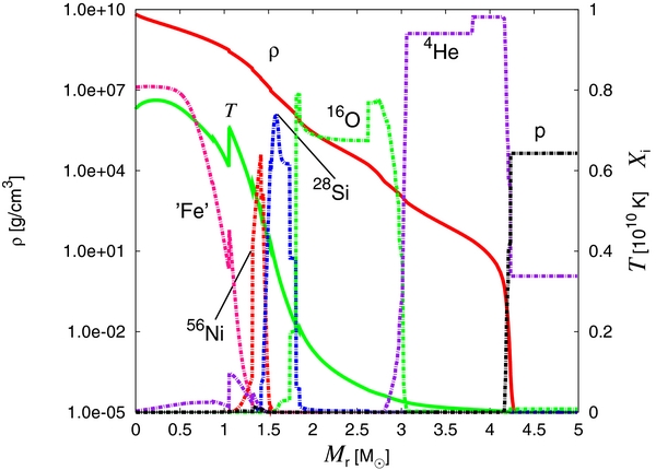
Figure 1. Initial profile of the 15 M☉ progenitor with an iron core with MFe = 1.4 M☉. The density (red solid line) and temperature (green solid line) as well as the mass fractions of some representative nuclei (solid dotted lines) are shown.
Download figure:
Standard image High-resolution image2.3. Step 1: 1D Simulation of the Infall of the Envelope
We now proceed to the description of the first step in the preparation of the initial models. The aim of this step is to sample the mass accretion rates as a function of time together with the changes in the structure and composition of the envelope. For this purpose, we perform a 1D simulation of the spherically symmetric implosion of the stellar envelope. We excise the interior within r = 60 km and replace it with the inner boundary, at which point we impose the free inflow condition. Since no bounce occurs in this simulation, no shock wave emerges. Note that what we need is the accretion rate and the structure outside the stalled shock wave, which would be produced and stalled somewhere inside the core in reality. The accretion rate and the structure are unaffected by what happens inside the shock wave since they are causally disconnected. The location of the inner boundary is chosen so that the accretion rate and the structure outside the stalled shock wave would always reside inside the shock wave.
We deploy 500 grid points to cover the region extending to r = 2 × 10⁵ km. This is large enough to ensure that matter outside the outer boundary does not move essentially for ∼ a second during this stage. The weak interactions are turned off for this computation, since they are indeed negligible in the infalling envelope. Note again that the computational results for the region that would be engulfed by the shock wave in reality are irrelevant and do not have any consequence on the results outside. Hence, neglecting neutrino heating and cooling is completely justified. The nuclear reactions for the 28 nuclei, on the other hand, are computed for the region with T < 7 × 10⁹ K to follow the change in chemical composition and take into account its influence on hydrodynamics during the implosion. The NSE composition is calculated for higher temperatures.
We show the results in Figure 2. In the upper panel, we show the mass accretion rate,  , as a function of radius for different te values, where te is the elapsed time from the beginning of collapse. One sees that the rarefaction wave generated by the inflow at the inner boundary propagates outward, triggering the infall of matter at large radii. After te ∼ 300 ms, the accretion rates at r ≲ 500 km become independent of radius. This observation implies that the flows in this region can be approximated by steady accretions. The region is actually expanding outward gradually. The lower panel shows the accretion rates at three different radii as a function of time. These rates agree with each other after te ∼ 300 ms. Before this time, on the other hand, the accretion rate is higher at smaller radii. There appears a peak at te ∼ 180 ms, which is rather insensitive to radius. From a comparison with realistic simulations (Janka et al. 2007), we find that this time roughly corresponds to the time of core bounce. We hence refer hereafter to the time elapsed from this point as the post-bounce time, i.e, tpb ≡ te − te(p), where te(p) denotes the time of the peak accretion rate. In the same panel, we also show the mass that has flown into the inner boundary by the given time. We refer to this mass as the PNS mass (MPNS). In the bottom panel, we present the time evolution of the mass accretion rate. We also indicate the evolution of the MPNS.
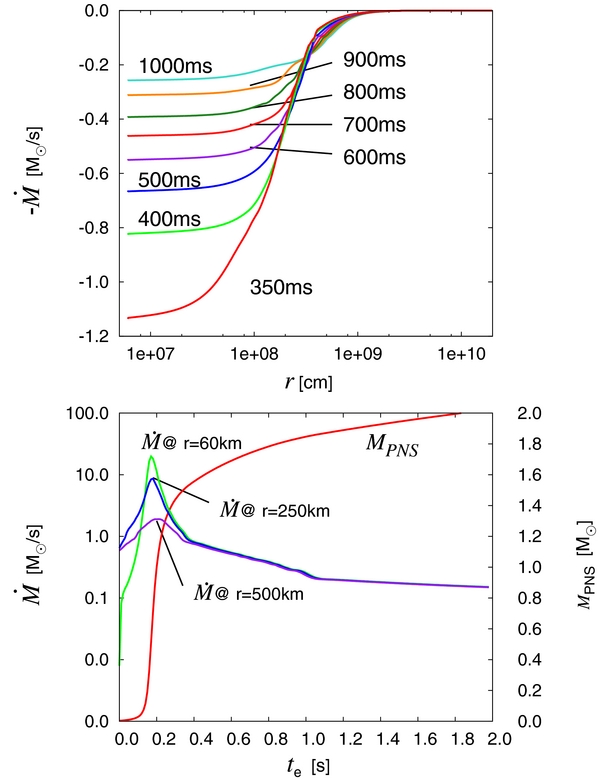
Figure 2. Characteristics of the mass accretion rates. The upper panel shows the radial profiles of  for different elapsed times, te. The lower panel displays the time evolution of
  at three different radii; the evolution of the proto-neutron star mass, MPNS, is also shown.
Download figure:
Standard image High-resolution imageThe evolution of the chemical composition, together with the density, velocity, and temperature, are displayed in Figure 3. In the left column, density and velocity are shown for three different post-bounce times (tpb). As time passes, the density at a fixed radius decreases monotonically, whereas the inflow velocity gets larger. The outward propagation of the rarefaction wave is also seen in the figure, which is exactly how the implosion of the envelope proceeds. In the right column, the chemical composition and temperature are presented for the same tpb. The temperature at a fixed radius is generally a decreasing function of time. It is observed that heavy elements are advected inward. In addition, the changes in composition due to nuclear burnings are also taken into account in this figure.
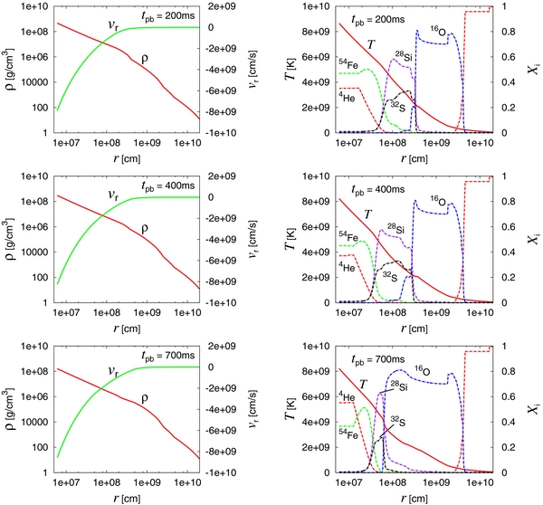
Figure 3. Evolution of the chemical composition, density, velocity, and temperature. In the left column, the density (red line) and velocity (green line) are displayed for three different times, tpb = 200, 400, and 700 ms, respectively. In the right column, the abundances of some representative nuclei (solid dotted lines) are shown with the temperature (solid line) for the same three times.
Download figure:
Standard image High-resolution imageWe employ these results not only at the next step of the preparation of initial conditions, which we will describe in the next section, but also in the simulations of the post-relaunch evolutions. We present the results of these simulations in Section 3.
2.4. Step 2: Search for Critical Luminosities
The purpose of this step is to construct the critical steady accretion flows with a standing shock wave for the mass accretion rates obtained in Step 1. It is important here to define unambiguously the critical point for a given accretion rate. In this paper, the critical point is meant for the highest luminosity with a steady accretion solution (Burrows & Goshy 1993). Instead, we define it to be the flow, in which the stalled shock wave is actually relaunched within a certain time. This is because the shock revival normally occurs because of hydrodynamical instabilities even in 1D before the luminosity above which no steady accretion is possible is reached. Hence, we determine the critical point hydrodynamically by following the growth of instabilities for initially spherically symmetric and steady accretion flows.
We hence adopt a two-step procedure. In the first step, we construct a sequence of spherically symmetric and steady accretion flows with a standing shock wave for a given mass accretion rate. We solve Equations (1)–(5) in 1D, dropping the Eulerian time derivatives. At the shock wave, we impose the Rankine–Hugoniot jump conditions. The nuclear reactions and weak interactions that are described in Section 2.2 are fully taken into account. The outer boundary of the computational domain is set at 500 km and the values of various quantities are taken from the results of step 1 at the times that correspond to the given mass accretion rates (see the bottom panel of Figure 2). At the inner boundary, which is placed according to Equation (8) with the post-bounce time obtained from the mass accretion rate, we impose the condition that the density is ρ = 1011 g cm−3. We cover the computational region with 300 grid points. As the neutrino luminosity is increased, the location of the standing shock wave is shifted outward and at some point the constant solution ceases to exist. As mentioned already, however, we do not need to evaluate this point, since the shock revival occurs earlier owing to the hydrodynamical instabilities. We do need to identify this point in the second step, however, and we refer to it as the critical point.
The hydrodynamical simulations are performed both in 1D and 2D in the second step. As mentioned just now, these computations are used to judge whether the spherically symmetric, steady accretion flows, which are obtained in the first step, induce shock revival due to the hydrodynamical instabilities. The nature of the instabilities is different between 1D and 2D: in 1D, radial oscillations become overstabilized at some luminosity, which is lower than the luminosity, at which the steady flow ceases to exist (Ohnishi et al. 2006; Fernández 2012). In 2D, on the other hand, the non-radial instability called SASI occurs even earlier on (Yamasaki & Yamada 2007). Hence, in reality the latter will be more important. We think that 1D models are still useful for understanding the physical processes that occur after the shock relaunch as well as elucidating the differences caused by the dimensionality of the hydrodynamics.
We solve Equations (1)–(5) numerically with all the time derivatives turned on. Both the input physics and radial grid are identical to those employed in the first step, in which the steady accretion flows are calculated. In 2D simulations, we employ 60 grid points in the θ direction to cover 180° and add random 1% perturbations to the radial velocity to induce SASI. In these simulations, we fix both the outer and inner boundary conditions and follow the evolution for 200 ms. If the shock wave reaches the outer boundary located at r = 500 km within this period, we judge that the shock is successfully revived. The reason we fix the boundary conditions is that if the shock revival occurs at a certain time, the instabilities should have reached the nonlinear stage by that time but the growth of the instabilities takes some time. For each mass accretion rate, we determine the minimum luminosity for the successful shock revival within a few percent and refer to it as the critical luminosity. In 1D, the shock relaunch is preceded by the growth of radial oscillations (not shown in the figure), whereas the non-radial modes with ℓ = 1, 2 are followed by the shock revival in 2D. Here, ℓ stands for the index of spherical harmonics in the expansion of unstable modes. In Figure 4, the critical luminosities are presented both for 1D and 2D as a function of the mass accretion rate. It is evident that the critical luminosity is a decreasing function of the mass accretion rate and it is reduced in 2D. Both of these results are well known (Ohnishi et al. 2006; Murphy & Burrows 2008).
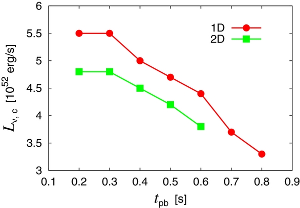
Figure 4. Critical neutrino luminosities in 1D and 2D as a function of the post-bounce time.
Download figure:
Standard image High-resolution image2.5. Step 3: Computation of Post-relaunch Evolution
In this section, we provide details of the 1D and 2D hydrodynamical simulations of post-shock-revival evolution. We continue the computations of Step 2 for the models with the critical luminosities. We first map the results to a larger mesh that covers the region extending from the neutrino sphere to a radius of r = 2 × 10⁵ km. In all 1D models, we computed the post-revival evolutions for ∼2 s, which is found to be long enough to estimate the explosion energy. In fact, we follow the evolutions for two 1D models until the shock reaches the stellar surface, which is located at r = 5 × 10⁸ km. In those simulations, we expand the mesh twice as the shock propagates outward. The inner boundary is also shifted to larger radii, to r = 103 km for the first re-gridding and to 104 km for the second expansion. These shifts avoid too severe Courant–Friedrichs–Lewy (CFL) conditions on the time step. We confirmed that these shifts of the inner boundary do not violate the energy conservation in ejecta by more than 0.1%. We also performed long simulations in a similar way (see Section 3.2) for three 2D models in order to determine the asymptotic ejecta mass accurately. In all simulations, we employ radial grid points non-uniformly (650 in 1D and 500 in 2D). In the 2D simulations, 60 grid points are distributed uniformly in the θ direction to cover the entire meridian section.
The outer boundary condition poses no problem this time, since it is located at a very large radius. We simply impose the free inflow/outflow condition there. The inner boundary conditions are a bit more difficult. We assume that the time evolution of the neutrino luminosity is given by

where texp is the time elapsed from the shock relaunch and Lν, c is the critical luminosity obtained in Step 2. We fix the density, pressure, and velocity at the ghost mesh point at the inner boundary when matter is flowing inward. When matter begins to flow outward, i.e., the transition to the neutrino wind phase occurs, those quantities are extrapolated from the innermost active mesh point to the ghost mesh point except when the entropy per baryon tends to be too high. In these cases, we put an upper bound of s = 100kB on the entropy per baryon and the density is adjusted. These prescriptions are applied to each angular grid point at the inner boundary for the 2D simulations.
We investigate seven 1D models, for which the stalled shock is relaunched at tpb = 200, 300, 400, 500, 600, 700, and 800 ms. Note that tpb has a one-to-one correspondence with the mass accretion rate, which is shown in Figure 2. Five 2D simulations are performed, in which the shock revival is assumed to occur at tpb = 200, 300, 400, 500, and 600 ms. See Figure 4 for the critical luminosities in these models. The input physics, such as nuclear and weak interactions, is the same as in the second step of step 2. The results of all the computations in this step will be presented in the next section, first for the 1D models and then for the 2D cases.
3. RESULTS
3.1. Spherically Symmetric 1D Models
3.1.1. The Evolution of the Fiducial Model
We first describe in detail the evolution of the 1D model, in which the shock relaunch is assumed to occur at tpb = 400 ms. This corresponds to the time at which the mass accretion rate is 0.53 M☉ s−1. The critical luminosity in 1D is 5 × 1052 erg s−1.
In Figure 5, we show the density, temperature, and mass fractions of representative nuclei as a function of radius for four different times. In the upper left panel, the profile at texp = 20 ms after the shock relaunch is displayed. The shock is still located around r = 500 km. The post-shock temperature is T ≳ 1 MeV, so high that the nuclei, flowing into the shock mainly 28Si, are decomposed to α particles. These particles are further disintegrated into nucleons immediately. The post-shock composition is perfectly described by NSE. At texp = 100 ms, the shock reaches r ∼ 2000 km but is still inside the Si layer as seen in the upper right panel of Figure 5. The post-shock matter is mainly composed of α particles, which are not disintegrated any more owing to the lower temperature, T ∼ 7 × 10⁹ K. Another 50 ms later, the shock enters the oxygen layer (see the lower left panel). Now 56Ni emerges just behind the shock wave. This is mainly due to the recombination of α particles, which will be evident shortly. The post-shock temperature is T ∼ 5 × 10⁹ K and matter is beginning to be out of NSE. In the lower right panel, we present the profile at texp = 500 ms. At this time, the temperature is T ∼ 2 × 10⁹ K and matter is completely out of NSE and the nuclear reactions yield mainly 28Si. For behind the shock wave, some α particles recombine to form 56Ni. Slightly later, all nuclear reactions are terminated behind the shock wave, since the temperature does not rise to high enough values by shock heating.
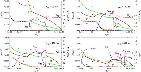
Figure 5. Density (red solid line), temperature (green solid line), and mass fractions of representative nuclei (solid dotted lines) for the 1D fiducial model as a function of radius at four different post-relaunch times, texp = 20, 100, 150, and 500 ms, respectively. The last snapshots show 56Ni production (purple) and α-rich freeze-out (blue). One can also see in the last panel 28Si production (dark green) by oxygen burning (magenta).
Download figure:
Standard image High-resolution imageIn Figure 6, we show the masses of protons, neutrons, α particles, 28Si, and 56Ni integrated over the region inside the shock wave as a function of texp for the 1D fiducial model. In accordance with the description in the previous paragraph, α particles are the main yield of nuclear reactions up to texp ∼ 100 ms. The depletion of neutrons after texp ∼ 50 ms implies that the nucleons are recombining to form α particles during this period. From texp ∼ 100 ms to texp ∼ 150 ms, on the other hand, α particles are diminished while 56Ni increases. This result means that the former recombines to the latter. After texp ∼ 150 ms, α particles cease to recombine any more and are frozen, and 56Ni and later 28Si are produced by nuclear burning. These results are obtained with the nuclear network with 28 nuclei (see Section 2.2). In order to confirm that it is large enough, we conduct a larger network with 463 nuclei as a post-processing calculation, employing the time evolutions of density, temperature, and electron fraction obtained from the simulation with the original network. The nickel and silicon masses are 0.140 M☉ and 0.068 M☉ for the larger network, respectively, whereas they are 0.151 M☉ and 0.071 M☉ for the standard case, respectively. Furthermore, the difference in the total mass of heavy nuclei with A ⩾ 48 is only 2.0 × 1.0−3 M☉ and the additional energy release from this difference is estimated to be less than 1.0 × 1049 erg. These results imply that the original network is appropriate.
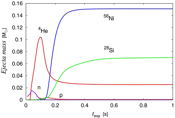
Figure 6. Ejecta masses of protons (dark red line), neutrons (purple line), α particles (red line), 28Si (green line), and 56Ni (blue line) integrated over the post-shock region, as a function of the elapsed time, texp, for the 1D fiducial model. No fall-back occurs and the masses of 56Ni and 28Si are determined as early as texp ∼ 500 ms.
Download figure:
Standard image High-resolution imageThe energy release from these nuclear reactions is presented in Figure 7. We time-integrate the energy production rate over the entire evolution as a function of mass coordinates. In so doing, we distinguish the contributions of the recombinations from those of the nuclear burnings. Moreover, the former is divided into two pieces, one of which comes from the recombinations in NSE and the other from those in non-NSE. In the interior (≲ 1.75 M☉), the recombinations start in NSE and end in non-NSE and hence there are two contributions. In the slightly outer layer up to ∼1.8 M☉, on the other hand, the recombinations occur in non-NSE conditions. Farther outside (≳ 1.8 M☉), the nuclear burning takes their place. In fact, the densities and temperatures of the matter in this region are inside the O-burning regime (see Figure 1 in Hix & Thielemann 1999). It is evident that the largest energy release comes from the recombinations that occur in NSE and the contributions of the nuclear burnings are rather minor even after being integrated over the mass coordinate for this particular model. This is a generic trend as will be shown later. There is a gap between ∼1.75 M☉ and ∼1.8 M☉. This is a region in which energy is not released but rather is absorbed. The main reaction in this region is the burning of 28Si to 56Ni. Some fraction of 28Si is disintegrated to α particles, however. Although the fraction of α particles is small, the mass difference between α particles and 28Si is much greater than that between 28Si and 56Ni. As a result, the energy consumed by the decomposition overwhelms the energy released by the burning.
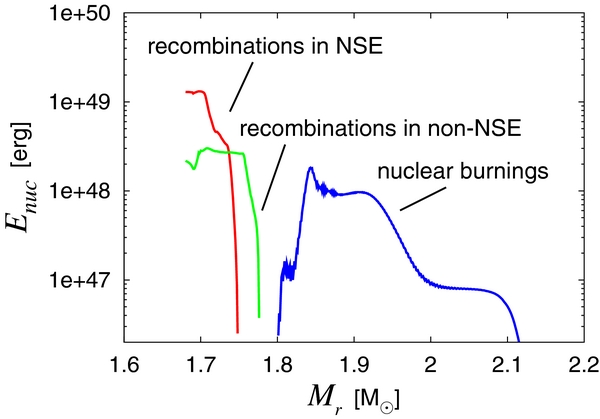
Figure 7. Total energy released by nuclear reactions as a function of mass coordinates. The size of the mass bin is 1.0 × 10⁻³ M☉. The energy production rate is obtained by integrating over the entire evolution. Mass bins being taken as three contributions, i.e., recombinations in NSE (red line), those in non-NSE (green line), and nuclear burnings (blue line).
Download figure:
Standard image High-resolution image3.1.2. The Evolution of the Diagnostic Explosion Energy
Now that we understand the evolution of density, temperature, chemical composition, and energy generation by nuclear reactions, we now turn our attention to the explosion energy. Following the conventional practice, we define the diagnostic explosion energy of provisional ejecta. At each grid point, the total energy density, etot, is given by

where ekin = 1/2ρv2 is the kinetic energy density, eint denotes the internal energy density, and egrav = ρ(Φ + Φc) stands for the gravitational potential energy density. We judge that the mass element at a certain grid point will be ejected if the total energy density is positive, etot > 0, and if the radial velocity is positive (vr > 0) at a given time. Then, the diagnostic explosion energy is defined as a function of time to be the sum of the total energy density times the volume over the ejecta, which has been determined previously.
The diagnostic explosion energy indeed changes with time. In the early phase of shock revival, neutrino heating is the main source of the diagnostic explosion energy. As the shock propagates outward, neutrino heating becomes inefficient, since the matter to be heated is also shifted to larger radii, where the neutrino flux is lower, and the luminosity itself becomes smaller as time passes. It is also important that nucleons, which are mainly responsible for the heating, are depleted as they recombine to α particles and heavier nuclei as the temperature decreases. After the neutrino heating subsides, nuclear reactions are the main energy source. As described in the previous section, the recombination of nucleons occurs first and the nuclear burnings take place later. After all the nuclear reactions terminate owing to low temperatures, the diagnostic explosion energy decreases slowly since matter, which is gravitationally bound and hence has negative specific energy, is swallowed by the shock wave. As the shock wave proceeds outward, this contribution becomes smaller and the diagnostic explosion energy approaches its asymptotic value, the actual explosion energy.
Figure 8 shows the time evolution of the diagnostic explosion energy for the 1D fiducial model, in which the shock is relaunched at tpb = 400 ms. The horizontal axis in the figure is the time elapsed from the shock relaunch, texp. The diagnostic explosion energy increases for the first ∼200 ms. Then it decreases gradually and becomes almost constant at texp ∼ 1 s. Also displayed in the figure are the individual contributions to the diagnostic explosion energy from neutrino heating and nuclear reactions. As described in the previous paragraph, neutrino heating is dominant over nuclear reactions initially up to texp ∼ 120 ms. Then, nuclear reactions become more important and raise the diagnostic explosion energy to ∼1051 erg at texp ∼ 200 ms in this particular case. As indicated by the colored lines in the figure, nuclear reactions are mainly recombinations until texp ∼ 150 ms. Nuclear burning follows until texp ∼ 300 ms. The asymptotic value of the diagnostic explosion energy is approached from above owing to matter being engulfed with negative energy by the outgoing shock wave.
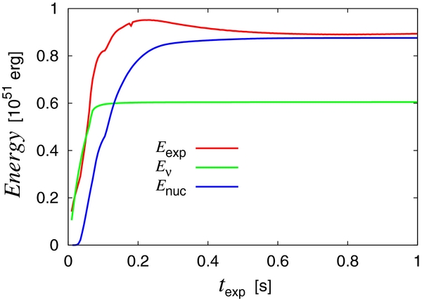
Figure 8. Time evolution of the diagnostic explosion energy for the 1D fiducial model. The individual contributions from neutrino heating (green line) as well as nuclear reactions (blue line) are also shown.
Download figure:
Standard image High-resolution imageIn order to confirm that the final explosion energy has been reached in the above computation, we continue to evolve this model until the shock wave reaches the stellar surface. We shift both the outer and inner boundaries as mentioned in Section 2.5 to avoid too severe CFL conditions at the innermost mesh point. The result is presented in Figure 9. It is clear that the diagnostic explosion energy is essentially constant for texp ≳ 1 s. Also shown in the figure is the result for another model, in which the shock relaunch is delayed until tpb = 800 ms. The accretion rate is ∼0.23 M☉ s−1 and the critical luminosity is ∼3.3 × 1052 erg s−1 for this 1D model. As is obvious from the figure, the asymptotic explosion energy is considerably smaller, ∼1.1 × 1050 erg, and we have to wait for ∼2 s before the diagnostic explosion energy settles to its asymptotic value. This is a generic trend: as the shock relaunch is delayed, it takes more time to reach the final explosion energy.
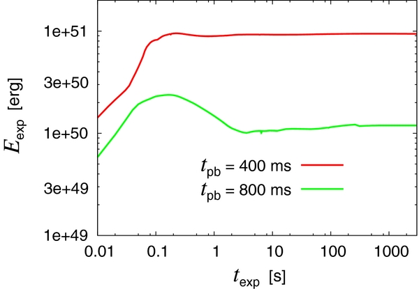
Figure 9. Long-term evolution of diagnostic explosion energies for the 1D fiducial model as well as for the model of the latest shock relaunch.
Download figure:
Standard image High-resolution image3.1.3. Systematics
In this section, we look at the results of other models to see how generic the findings of our fiducial model are. In Figure 10, we show the asymptotic values of the diagnostic explosion energy for different models as a function of the shock-relaunch time. We can clearly see that the explosion energy is a monotonically decreasing function of the shock-revival time. This result is mainly due to the fact that the mass of accreting matter decreases as time passes; the finding is not unexpected (see, e.g., Scheck et al. 2006). We stress, however, that this is the first clear demonstration of taking into account nuclear reactions and EOS in sufficiently long computations. We confirm that the diagnostic explosion energy asymptotes to a constant value.

Figure 10. Asymptotic values of the diagnostic explosion energy for all 1D models.
Download figure:
Standard image High-resolution imageAlso shown in the figure are the individual contributions to the diagnostic explosion energy from nuclear reactions and neutrino heating. Both of these processes also decrease as the shock revival is delayed. It is found, however, that the contribution of nuclear reactions diminishes more rapidly. This is simply due to the fact that the temperature increase due to the shock passage is smaller in weaker explosions. Note that the explosion energy is smaller than the sum of the two contributions, since the accretion of gravitationally bound matter contributes negatively to the explosion energy, as mentioned already. It should also be emphasized that the recombination energy eventually originates from neutrino heating because the recombinations are necessarily preceded by the endothermic dissociations of heavy nuclei that exist prior to collapse. The consumed energy is replenished by neutrinos. Neutrino heating also plays a vital role in pushing the post-bounce configuration to the critical point and further heating up matter until it becomes gravitationally unbound in the earliest phase of shock revival.
In Figure 11, we further divide the contribution of nuclear reactions into those from the recombinations in and out of NSE as well as those from nuclear burning. Roughly speaking, the re-assembly of nucleons into α particles occurs in recombination in NSE and further recombinations to heavier nuclei proceed in the environment out of NSE. As can be seen, all the contributions again decline as the shock relaunch is delayed. Regardless, the recombination that occurs in NSE is the greatest contributor. The recombinations, both in and out of NSE, decline more rapidly than nuclear burning and the latter contributes more than the recombination out of NSE for the model. Out of NSE, the shock revival occurs at the latest time (tpb = 800 ms) and the weakest explosion is obtained. The reason why nuclear burning declines more slowly is that the temperatures obtained by shock heating are roughly proportional to the quarter power of the explosion energy.

Figure 11. Individual contributions to the explosion energy from nuclear recombinations in NSE, non-NSE, and nuclear burning.
Download figure:
Standard image High-resolution imageNext, we turn our attention to the synthesis of 56Ni, one of the most important observables in the supernova explosion. The synthesized mass of 56Ni is correlated with the explosion energy (Hamuy 2003): the greater the explosion energy, the more 56Ni is produced. This is demonstrated in Figure 12. In the upper panel, we again present the asymptotic values of the diagnostic explosion energy, which we simply refer to as the explosion energy. These values are a function of the mass accretion rate at shock relaunch. The corresponding shock-relaunch times are given in the figure. In the lower panel, the mass of 56Ni in the ejecta is also displayed as a function of the mass accretion rate at shock relaunch. The ejecta was defined earlier to be the collection of the mass elements that have positive total energy density and radial velocity (see Section 3.1.2). The positive correlation between the explosion energy and the mass of 56Ni in the ejecta is evident.
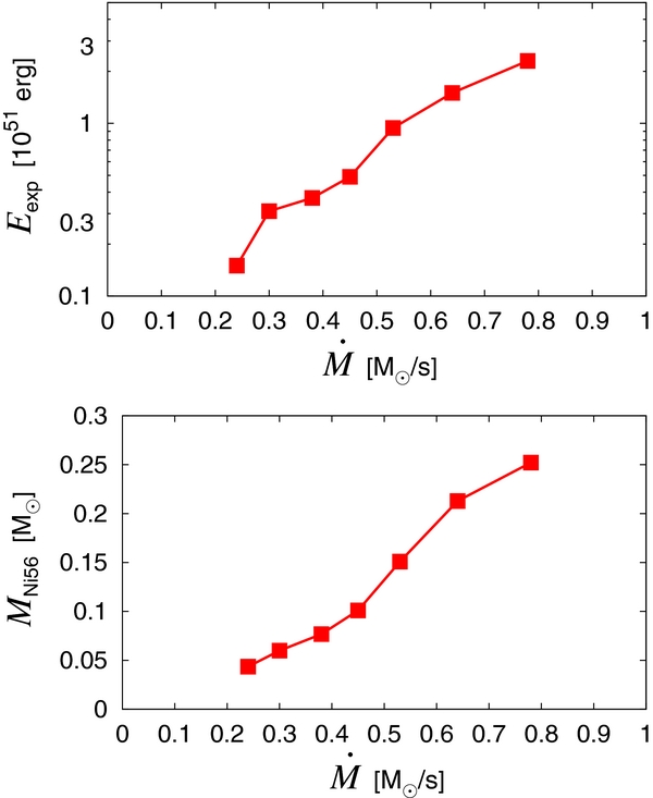
Figure 12. Explosion energies and 56Ni masses for all the 1D models.
Download figure:
Standard image High-resolution imageIn fact, 56Ni may be produced too much in these 1D models. The canonical explosion energy (∼1051 erg) is attained only by the models that relaunch the stalled shock wave relatively early (tpb ≲ 400 ms). On the other hand, the masses in the ejecta of 56Ni synthesized for all these models are ≳ 0.15 M☉, which is substantially larger than the values estimated from observations (≲ 0.1 M☉; Smartt et al. 2009a). Note that the mass of 56Ni ejected by SN1987A is estimated to be ∼0.07 M☉. This value corresponds to a shock-relaunch time of tpb ∼ 600 ms in our 1D model; this rather late shock revival gives only a weak explosion of ∼0.4 × 1051 erg, smaller than the most likely explosion energy of SN1987A derived observationally (0.9 × 1051 erg; Kasen & Woosley 2009). It is true that both the observational estimates and the theoretical predictions presented here have uncertainties. In fact, the neutrino transport as well as the evolution of PNSs, which are neglected and simply parameterized in this paper, are the main sources of uncertainties in the results shown above. We believe, however, that the general trends would be unchanged even if more sophisticated treatments were adopted. The above argument hence may be regarded as yet another reason why we do not believe that the 1D neutrino heating works.
To better understand the origin of the overproduction of 56Ni, we have performed an ordinary calculation of explosive nucleosynthesis as a post-process for the densities, temperatures, and electron fractions obtained for the models presented above. In so doing, the so-called thermal bomb method, in which thermal energy is deposited initially in the innermost region, is employed (Hashimoto 1995). The explosion energy and mass cut are chosen so that they agree with those of the original models. Interestingly, the calculation of explosive nucleosynthesis consistently produces smaller amounts of 56Ni, as given in Table 1. In fact, the fiducial model reproduces the observational estimate for SN1987A much better; this agreement may just be a coincidence, though. Figure 13 compares the distributions of peak temperatures between the 1D fiducial model and the corresponding thermal-bomb model. It is clear that the fiducial model has a larger fraction of mass elements that achieve high enough temperatures to produce 56Ni. The neutrino heating mechanism seems to require a greater thermal energy to unbound the accreting envelope. This result may also serve as a warning against employing the thermal-bomb method in the explosive nucleosynthesis calculations.

Figure 13. Comparison of the distributions of peak temperature between the 1D fiducial model and the corresponding thermal-bomb model. The total mass of the matter that has a peak temperature higher than T9 = 5 is 1.89 × 10⁻¹ M☉ for the 1D model and 1.20 × 10⁻¹ M☉ for the themal-bomb model.
Download figure:
Standard image High-resolution imageTable 1. Comparison with an Ordinary Explosive-nucleosynthesis Calculation
| Shock Relaunch Time | Explosion Energy | Proto-neutron Star Mass | 56Ni Mass | |||
|---|---|---|---|---|---|---|
| (ms) | (1051 erg) | (M☉) | (M☉) | |||
| 1D Model | Thermal Bomb | 1D | Thermal Bomb | 1D | Thermal Bomb | |
| 300 | 1.50 | 1.50 | 1.60 | 1.59 | 0.21 | 0.15 |
| 400 | 0.95 | 0.94 | 1.67 | 1.64 | 0.15 | 0.086 |
| 500 | 0.50 | 0.60 | 1.70 | 1.73 | 0.10 | 0.043 |
Download table as: ASCIITypeset image
In fact, Young & Fryer (2007) discussed the uncertainty in nucleosynthetic yields with 1D spherically symmetric explosion models and showed that 56Ni evaluated with the piston-driven model (Eexp = 1.2 × 1051 erg) is larger by a factor of 2–3 than that with the thermal-bomb model (Eexp = 1.5 × 1051 erg) with the same remnant mass. Our 1D neutrino-driven explosion models may be closer to the piston-driven explosion model than to the thermal-bomb explosion model.
3.2. Axisymmetric 2D Models
In this section, we focus on the effects of dimension. In Section 2.4, we already showed that the critical neutrino luminosity is lower in the axisymmetric 2D models than in the spherically symmetric 1D model for the same accretion rate at the shock relaunch. Performing 2D simulations further in step 3, we are concerned with how and how much the results we obtained for the 1D models so far are modified for the 2D cases.
The input physics for 2D simulations is essentially the same as for the 1D model except for the perturbations added to the radial velocities with random magnitudes up to 1% at the beginning of step 2. We have investigated the models in which the stalled shock wave is relaunched at the post-bounce times of tpb = 200, 300, 400, 500, and 600 ms. For the models with tpb = 400, 500, and 600 ms, we further extend the domain twice up to r = 2 × 10⁷ km as already mentioned. This is necessary to determine the mass of the matter that eventually falls back. It turns out that the model with tpb = 600 ms fails to explode, with all the shocked matter falling back before the shock wave reaches the He layer. We also tested the numerical convergence in the model with tpb = 400 ms by increasing the numbers of radial or angular grid points. We found that the higher radial resolution (700 mesh points instead of 500) does not make much difference. Incidentally, this is also the case in 1D. On the other hand, the finer angular mesh (90 grid points instead of 60) yields an explosion energy and 56Ni abundance that are 16% and 10% larger than those for the standard resolution, respectively.
3.2.1. Dynamics of Aspherical Shock Revival
We first look at the post-relaunch dynamics of the tpb = 400 ms model, which is the 2D counterpart to the 1D fiducial model. As shown in Figure 14, which displays the contours of entropy per baryon and the mass fraction of 56Ni, the shock expansion is highly aspherical, which was also demonstrated by Kifonidis et al. (2006), Ohnishi et al. (2006), Scheck et al. (2006, e.g.,). The shock front is elongated in the direction of the symmetry axis. The shock propagates more rapidly in the northern hemisphere, whereas matter attains a higher entropy per baryon in the opposite hemisphere. These features conform with the dominance of ℓ = 1, 2 modes owing to SASI. Here, ℓ stands for the index of the Legendre polynomials, which are included in the eigenfunctions of linearly unstable modes.

Figure 14. Contours of entropy (left panel) and mass fraction of 56Ni (right panel) at texp = 400 ms for the 2D model, in which the stalled shock revives at tpb = 400 ms.
Download figure:
Standard image High-resolution imageAs mentioned in Section 2.4, the shock revival occurs at a lower luminosity in the 2D model (Lc = 4.2 × 1052 erg s−1) than in the 1D counterpart (Lc = 5.0 × 1052 erg s−1). Unlike the 1D case, some matter continues to accrete, forming downdrafts, particularly in the equatorial region. This process continues until much later times after the shock revival. As a consequence, the (baryonic) mass of the neutron star is larger in the 2D case (∼2.1 M☉) than in the 1D case (∼1.65 M☉). This is actually a generic trend as shown later (see Figure 17). Another interesting feature found in the 2D model is the distribution of maximum temperatures that each mass element attains, which is obtained from the Lagrangian evolution of tracer particles distributed in the ejecta. Figure 15 shows the result in a histogram. It is evident that the mass that reaches T = 5 × 10⁹ K is larger in 1D than in 2D. In the same figure, we also show the distribution of electron fraction, Ye(NSE), which is estimated when T becomes the boundary value of NSE, or 7 × 10⁹ K. Note that Ye(NSE) is useful for the diagnosis of nuclear yields in ejecta. In the 1D case, there exist too massive ejecta with Ye(NSE) ⩽ 0.49, which will produce unacceptable amounts of neutron-rich Ni isotopes and 64Zn compared with the solar abundances as shown by Fujimoto et al. (2011). Their overproduction of the slightly neutron-rich ejecta with Ye(NSE) ⩽ 0.49 in the 1D case disappears in the 2D case owing to more efficient neutrino interactions. Multi-dimensional models are therefore preferable with regard to understanding the Galactic chemical evolution of isotopes, although these models may depend on the treatment of neutrino transfer.
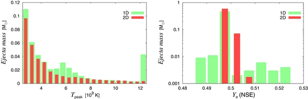
Figure 15. Comparison of the distributions of peak temperatures Tpeak (left panel) and Ye(NSE) (right panel) between the 1D fiducial model and its 2D counterpart. The total mass of the matter that has the peak temperature higher than T9 = 5 is 1.89 × 10⁻¹ M☉ in 1D and 9.62 × 10⁻² M☉ in 2D.
Download figure:
Standard image High-resolution imagePost-relaunch evolution is a bit different between the models with the earlier (tpb = 200 and 300 ms) and later (tpb = 500 and 600 ms) relaunch. As shown in Figure 16, SASI is always dominated by the ℓ = 1, 2 modes, making the shock front rather prolate generically with a marked equatorial asymmetry. In the models with the earlier shock revival, the shock front is nearly isotropic, whereas in the models with the later shock relaunch, the matter expansion is highly anisotropic with large portions of post-shock matter continuing to accrete. The difference seems to have an origin in the difference of the steady states obtained in step 2. In the former, the shock radii are large and the post-shock flows are slow. As a consequence, the matter in the gain region is heated rather homogenously in the subsequent evolutions. For the latter, on the other hand, the gain region is narrow and the post-shock flows are faster, which tends to enhance inhomogeneites in the subsequent heating, leading to the localized expansion.

Figure 16. Post-shock-relaunch distributions of entropy per baryon in the meridian section for all the 2D models at texp ∼ 0.25 s.
Download figure:
Standard image High-resolution imageThe accretion continues until long after the shock is relaunched. The resultant mass of the neutron star is larger in 2D models than in 1D models as pointed out already for the fiducial model and now shown in Figure 17. As the shock revival is delayed and the critical luminosity decreases with a decreasing mass accretion rate, the post-relaunch evolution becomes slower as in 1D. This is even more so the case for the 2D models, for which the critical luminosity is smaller than for 1D models owing to hydrodynamical instabilities (see Figure 4). How these hydrodynamical features affect the explosion energy and nickel mass is our primary concern and will be addressed in the next section.
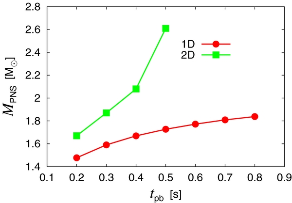
Figure 17. Comparison of the masses of proto-neutron stars at the end of computations between the 1D and 2D models.
Download figure:
Standard image High-resolution image3.2.2. Diagnostic Explosion Energies and Masses of 56Ni in the Ejecta
The diagnostic explosion energy is shown in Figure 18 as a function of texp for the 2D fiducial model, in which the stalled shock wave is relaunched at either tpb = 300 or tpb = 400 ms. This model is the counterpart to the 1D fiducial model. Also presented are the individual contributions from neutrino heating and nuclear reactions. As in the 1D fiducial model (see Figure 8), the neutrino heating is effectively closed at texp ∼ 100 ms. By this time, the shock front has reached r ≳ 2000 km, which is far enough from the PNS for the neutrino flux to become negligibly small. After the freeze-out of neutrino heating, the diagnostic explosion energy increases via nuclear reactions such as the recombination of 4He to heavier nuclei in the early phase and the Si and O burnings later on as shown in Figure 19. This figure shows the masses of n, p, 4He, and α particles, 28Si and 56Ni as a function of time.

Figure 18. Time evolution of the diagnostic explosion energy for the 2D models, in which the shock is relaunched at tpb = 300 ms (solid line) and tpb = 400 ms (solid dotted line).
Download figure:
Standard image High-resolution image
Figure 19. Time evolution of the masses of n, p, 4He, 28Si, and 56Ni as a function of texp for the models with tpb = 300 (left panel) and 400 ms (right panel).
Download figure:
Standard image High-resolution imageThe diagnostic explosion energies become almost constant at texp ∼ 600 ms in these models and the masses of 56Ni reach their maximum values around texp ∼ 300 ms. These features are essentially the same as what we observed for the 1D counterpart (Figures 6 and 8). However, big differences appear after texp = 300 ms in the masses of the heavy elements between the 1D and 2D models: significant fall-backs occur in 2D as can be seen in Figure 19. Incidentally, the ratio of the kinetic to internal energies in the ejecta is (Ekin/Eint) ∼ 4 at texp = 1000 s for all the exploding models.
Figure 20 shows the explosion energies for all the 2D models compared with those for the 1D models. It is a general trend that the explosion energy is a monotonically decreasing function of the shock-relaunch time although the gradient is much steeper in 2D. It is also interesting that the explosion for a given shock-relaunch time is similar between 1D and 2D models provided that the shock revival is early enough to give an explosion energy of 1051 erg. This may imply that it is the mass accretion rate that primarily determines the canonical explosion energy. It should be noted, however, that the critical luminosity for a given mass accretion rate is smaller in 2D than in 1D (see Figure 4). For a given neutrino luminosity, the explosion energy is hence larger in 2D except for a very weak explosion by the late shock relaunch. This is the advantage of non-spherical hydrodynamics that is commonly mentioned in the literature. For the model with tpb = 500 ms, the explosion energy is much smaller than for the 1D counterpart. No explosion is obtained in the model with tpb = 600 ms owing to the significant fall-back.
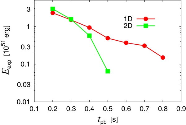
Figure 20. Comparison of the explosion energies between the 1D and 2D models.
Download figure:
Standard image High-resolution imageIn Figure 21, we present the individual contributions to the explosion energy from neutrino heating and nuclear reactions for both the 1D and 2D models. This figure should be compared with Figure 10. It is evident that both contributions from neutrino heating and the nuclear reactions drop much more quickly in 2D than in 1D as the shock revival is delayed; the contribution of the nuclear reactions decreases faster than that of neutrino heating and, as a consequence, the former is dominant only for the models with earlier shock relaunches (tpb ≲ 300 ms). It is also interesting that the decay of the explosion energy is accelerated once the contribution of the nuclear reactions ceases to be dominant. It thus seems that the energy release by nuclear reactions is an important ingredient for robust explosions. The reduced contribution from the nuclear reactions is directly related to the decrease of the mass elements in the ejecta that attain high peak temperatures, which we have pointed out already for the fiducial model (see Figure 15), as well as with the fall-back in the 2D models. These reductions are slightly compensated for by the reduction in the (negative) contribution from the gravitational energy of accreting matter that is swallowed in the ejecta. This is another consequence of the fact that the accretion continues in 2D even after the shock is relaunched and not all accreting matter is added to the ejecta.

Figure 21. Individual contributions of neutrino heating and nuclear reactions to the explosion energy for all the 1D and 2D models.
Download figure:
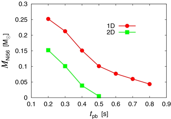
Standard image High-resolution imageThe reduced contribution to the explosion energy from nuclear reactions is also reflected in the production of 56Ni (Figure 22). It is apparent that the mass of 56Ni as a function of the shock-relaunch time is always smaller in 2D than in 1D. It should be noted that the 1D models tend to overproduce the nickels; as discussed in Section 3.1.3, if the typical mass of 56Ni in the ejecta of CCSNe is MNi ≲ 0.1 M☉ as observations seem to indicate (Smartt et al. 2009a), the 1D models require that the shock should be relaunched later than tpb ∼ 500 ms. This requirement implies a rather weak explosion (Eexp ≲ 0.5 × 1051 erg); however, no 1D model can provide both the explosion energy and nickel mass in the appropriate range. In the 2D models, on the other hand, this problem is lessened. Indeed, the explosion energy is large enough if the shock relaunch occurs earlier than tpb ∼ 400 ms, the nickel is not over-produced, and the shock is revived later than tpb ∼ 300 ms. Although it is an entirely different issue whether and how the critical luminosity is obtained, this range of shock-relaunch times, tpb ∼ 300–400 ms, may be regarded as the appropriate time for shock revival. It is convenient that the 2D models have an "allowed" range, since the hydrodynamics are inevitably non-spherical owing to the hydrodynamical instabilities. Whether three-dimensional hydrodynamics, which are the reality, alter the result for 2D models will be an important issue to be studied in the future.
Figure 22. Comparison of 56Ni masses in the ejecta between the 1D and 2D models.
Download figure:
Standard image High-resolution image
Comparing the abundances in SN ejecta and those in the solar system may possibly recover a similar allowed range of shock-relaunch times. Fujimoto et al. (2011) performed detailed nucleosynthetic calculations for the ejecta of an SN explosion from a 15 M☉ progenitor (Woosley & Weaver 1995). These calculations were based on simulations of a neutrino-driven aspherical explosion, which employed a hydrodynamic code similar to the one used in the present study but neglecting the energy generation through nuclear reactions. These authors showed that the explosions with tpb ∼ 200–300 ms give Eexp and M(56Ni) in the allowed range and that the abundances in the ejecta are similar to those in the solar system. Detailed nucleosynthesis studies taking into account energy generation via nuclear reactions will be interesting, since the feedback, which elevates entropy in the ejecta, will possibly enhance the amounts of 56Ni and 44Ti. These elements are slightly and highly underproduced in Fujimoto et al. (2011), respectively.
4. SUMMARY AND DISCUSSION
We have investigated with numerical experiments in 1D and 2D the post-shock-relaunch evolution in the neutrino heating mechanism. Taking into account the fact that the shock revival should occur somewhere on the critical line in the  diagram (but exactly where is rather theoretically uncertain at present), we have treated the luminosity (or equivalently the mass accretion rate) at the shock relaunch as a free parameter that we vary rather arbitrarily. Only the post-bounce phase has been computed and we have discarded the central region (r ≲ 50 km) and replaced it with the prescribed boundary conditions. We have also neglected neutrino transport entirely and have employed the light bulb approximation. The shock revival is hence induced by requiring a critical luminosity at the inner boundary.
The critical luminosity itself has also been determined by hydrodynamical simulations, since the onset of hydrodynamical instabilities, and not the non-existence of the steady state, dictates the shock revival. The mass accretion rate as a function of time is obtained from the simulation of the gravitational implosion of a massive star envelope. We have adopted a realistic 15 M☉ progenitor provided by Woosley & Heger (2007). In these computations, we have consistently taken into account the nuclear reactions among 28 nuclei that include 14 α nuclei as well as their feedback to hydrodynamics. As a result, we have confirmed that the critical luminosity is a monotonically decreasing function of the shock-relaunch time (or equivalently a monotonically increasing function of the mass accretion rate) and that 2D dynamics reduce the critical luminosity compared with 1D dynamics. This is due to the non-radial hydrodynamical instabilities and the resultant enhancement of neutrino heating in the former case.
After re-mapping, we have continued the simulations until long after shock revival. In fact, for some 1D models, we have followed the post-shock-relaunch evolution up to the shock breakout of the stellar surface, confirming that the diagnostic explosion energy has approached the asymptotic value much earlier. This finding confirms that the shorter computation times for other models are indeed sufficient. We have employed the same set of input physics as in the simulations for the setup of initial conditions. Integrating the source terms in the equation of energy conservation, we have evaluated the individual contributions from neutrino heating and nuclear reactions to the explosion energy. In doing so, we further divide the latter into the contributions from the recombinations in and out of NSE as well as from nuclear burnings. The axisymmetric 2D simulations have been performed to elucidate the effect of multi-dimensionality on the outcome.
What we have found in these model computations can be summarized as follows.
- 1.Immediately after shock relaunch, neutrino heating is the dominant source of explosion energy but is terminated before long as the shock propagates outward. Then, nuclear reactions become dominant, with the recombination of nucleons to α particles under the NSE condition occurring first. As the temperature decreases, the NSE is no longer satisfied. The recombination of α particles to heavier elements proceeds mainly in this non-NSE state. When the temperature decreases further, nuclear burnings of silicon and oxygen take place in the matter that flows into the shock wave. Matter that flows into the shock wave contributes negatively to the explosion energy, since it is gravitationally bound.
- 2.The final explosion energy is a monotonically decreasing function of the shock-relaunch time (or equivalently an increasing function of the mass accretion rate at shock relaunch), irrespective of the dimensionality of the hydrodynamics. There is no big difference between 1D and 2D for the same mass accretion rate at the shock relaunch as long as it occur earlier than tpb ≲ 300 ms and the explosion is robust. The late relaunch in 2D leads to a highly anisotropic expansion of matter with a large portion of the post-shock matter still accreting, which then yields very weak explosions, or none at all. This implies that the mass accretion rate is the primary factor determining the canonical explosion energy. Since the critical neutrino luminosity for a given mass accretion rate is lower in 2D than in 1D, the explosion energy for a given neutrino luminosity is larger except for a very weak explosion.
- 3.As the shock relaunch is delayed, the diagnostic explosion energy takes longer to reach the asymptotic value. In our 1D fiducial model, in which the stalled shock is revived at tpb = 400 ms and we obtain the explosion energy of Eexp ∼ 1051 erg, the diagnostic explosion energy attains the asymptotic value in texp ∼ 600 ms whereas it takes ∼2 s for the model in which the shock relaunch is assumed to occur at tpb = 800 ms and the explosion energy is as low as ∼1050 erg. A similar trend is also observed in the 2D models except for the case with tpb = 600 ms, in which no explosion occurs.
- 4.In 1D, the nuclear reactions always overwhelm the neutrino heating. The difference becomes smaller as the shock relaunch is delayed. For the nuclear reactions, the recombination of nucleons to α particles that occurs mainly under the NSE condition is the dominant contributor, followed by the recombination of α particles to heavier elements in the non-NSE condition. Nuclear burnings provide the smallest contribution except for the weakest explosion, which occurs for the latest shock relaunch. In that case, the nuclear burnings beat the recombinations in non-NSE. In 2D, on the other hand, the neutrino heating and nuclear reactions provide comparable contributions to the explosion energy with the latter being larger in stronger explosions and the latter being weaker in weaker explosions. Note, however, that the rather small contribution of neutrino heating is deceptive in the sense that it is the ultimate source of the energy obtained from the nuclear recombinations and that it is crucial to set the stage for shock revival. Shock revival is not accounted for in the diagnostic explosion energy.
- 5.In the 1D models, nickels are overproduced owing mainly to the larger mass that achieves higher peak temperatures compared with the ordinary calculation of explosive nucleosynthesis in post-process. In fact, there is no 1D model that produces typical values for the explosion energy and the nickel mass simultaneously. Given observational and theoretical uncertainties, we are not sure how serious a problem this is for the moment. One may consider, however, that this is yet another reason to abandon the 1D neutrino heating model. In 2D, on the other hand, this problem is solved, opening up the allowed region in the shock-relaunch time around tpb ∼ 300–400 ms, which produces an explosion energy and nickel mass in the appropriate range. This happens mainly in 2D because the mass of matter in the ejecta that attains high enough peak temperatures is smaller and the fall-back is significant. This is in turn related to the fact that the expansion and accretion occur simultaneously in 2D, which is indeed reflected in the mass of the PNS. The PNS mass is larger in 2D at any post-bounce time.
In the present paper, we have employed the single 15 M☉ progenitor model, which we think is one of the most representative for producing typical type IIP CCSNe. Very recently, Ugliano et al. (2012) reported a possible stochastic nature in the outcome of the shock revival in the neutrino heating mechanism based on systematic 1D hydrodynamical simulations. Although the stochasticity is less remarkable in the low-mass end, it is hence mandatory to extend the current work to other progenitors and see how generic our findings obtained in this paper are (Y. Yamamoto et al., in preparation). 3D models are also a top priority in future work, since we know that 3D SASI is qualitatively different from the 2D SASI we have studied in this paper (Iwakami et al. 2008). It should also be recalled that Nordhaus et al. (2010) claimed that shock revival is even easier in 3D than in 2D, although controversies are still continuing (Hanke et al. 2012). If the critical luminosity is much lower in 3D than in 2D, the yield of 56Ni may be reduced further in 3D. The complex flow patterns also have some influence on the nickel yield. We are particularly concerned with how the allowed region in the shock-relaunch time that is opened in 2D is modified in 3D. The relative importance of nuclear reactions for the explosion energy compared with neutrino heating is the highest in 1D. We are certainly interested in how these proportions may or may not change in 3D.
One of the greatest uncertainties in the present study is the effect of the inner boundary condition that is imposed by hand. The artificial treatment employed in this paper results in a total mass injection from the inner boundary of about 7 × 10⁻³ M☉ in the 1D fiducial model. This injection contributes 2%–3% to the explosion energies and the 56Ni masses. Although this may be a slight underestimate (Arcones et al. 2007), we believe that better treatments will not change the conclusion of this paper qualitatively. The eventual answer should come from fully consistent simulations of the entire core, though. It is also true that the simple light bulb approximation adopted in this paper does not accurately account for accretion luminosities, in particular their correlations with temporally varying accretion rates as well as the differences between 1D and 2D. Hence, the appropriate treatment of the neutrino transport, which is neglected completely in this paper, will be critically important. These caveats notwithstanding, we believe that the results obtained in this paper are useful for understanding the post-shock-relaunch evolution in the neutrino heating mechanism, particularly how the diagnostic explosion energy approaches the final value. One of the goals of our project is to investigate, a way to estimate the explosion energy from the early stage of post-shock-revival evolution, since realistic simulations may not be feasible for a few seconds after shock relaunch. More systematic investigations will be crucial for realizing this goal.
This work is partly supported by a Grant-in-Aid for Scientific Research from the Ministry of Education, Culture, Sports, Science and Technology of Japan (Nos. 19104006, 21540281, 24740165, 24244036, 22540297) and the HPCI Strategic Program of Japanese MEXT.