


ABSTRACT
The first stars to form in the universe are believed to have distribution of masses biased toward massive stars. This contrasts with the present-day initial mass function, which has a predominance of stars with masses lower than 1 M☉. Therefore, the mode of star formation must have changed as the universe evolved. Such a transition is attributed to a more efficient cooling provided by increasing metallicity. Especially dust cooling can overcome the compressional heating, which lowers the gas temperature thus increasing its instability to fragmentation. The purpose of this paper is to verify if dust cooling can efficiently cool the gas, and enhance the fragmentation of gas clouds at the early stages of the universe. To confirm that, we calculate a set of hydrodynamic simulations that include sink particles, which represent contracting protostars. The thermal evolution of the gas during the collapse is followed by making use of a primordial chemical network and also a recipe for dust cooling. We model four clouds with different amounts of metals (10−4, 10−5, 10−6 Z☉, and 0), and analyze how this property affect the fragmentation of star-forming clouds. We find evidence for fragmentation in all four cases, and hence conclude that there is no critical metallicity below which fragmentation is impossible. Nevertheless, there is a clear change in the behavior of the clouds at Z ≲ 10−5 Z☉, caused by the fact that at this metallicity, fragmentation takes longer to occur than accretion, leading to a flat mass function at lower metallicities.
Export citation and abstract BibTeX RIS
1. INTRODUCTION
Many theoretical models for the first stars to be formed in universe, the Population III (Pop III) predict that the stellar mass spectrum is dominated by massive objects in the range of tens to hundreds of solar masses (e.g., Abel et al. 2002; Bromm et al. 2002; O'Shea & Norman 2007; Yoshida et al. 2008; Hosokawa et al. 2011). Recent works have shown that low-mass stars can also be formed, albeit with characteristic masses still above the solar value (Clark et al. 2011a, 2011b; Greif et al. 2011, 2012; Smith et al. 2011; Stacy et al. 2010, 2012). In addition to that, observational data require a "top heavy" initial mass function (IMF) to explain the characteristics of some Galactic globular clusters (Marks et al. 2012; Kroupa et al. 2012), and also the high fraction of extremely metal-poor stars that are C-rich (Suda et al. 2012).
On the contrary, the present-day IMF is dominated by low-mass stars (Kroupa 2002; Chabrier 2003). This indicates that star formation changed from a mode that favors massive stars in the early universe to the mode in which the stars have masses lower than the solar value, which we observe today.
When gas clouds collapse, thermal energy is generated due to the compressive heating. If the collapse is adiabatic, then the critical mass for fragmentation remains constant with increasing density. By contrast, when this thermal energy can be dissipated by the emission of photons, then the critical mass for fragmentation drops as the density gets larger.
Moreover, for the metal-free case, the most important coolant is molecular hydrogen emission. In this case, numerical simulations show that the distribution of stellar masses should favor massive stars (Nakamura & Umemura 1999, 2001, 2002; Abel et al. 2002; Bromm et al. 2002; O'Shea & Norman 2007; Yoshida et al. 2008; Smith et al. 2011). Since H2 cooling is not efficient for low temperatures (T < 200 K) and high densities (n > 104 cm−3), the Jeans mass at such conditions can be up to three orders of magnitude higher than in present-day molecular clouds.
For the clouds enriched with the first metals, the gas can cool to lower temperatures and higher densities. Therefore, the characteristic fragment mass is expected to be lower. It has been proposed that this extra cooling provided by the metals could boost fragmentation and cause the transition in the star formation mode. This also suggests that the mode of star formation changes at a critical fraction of metals Zcrit.
The most important coolants at very low metallicities are dust (e.g., Schneider et al. 2002, 2006, 2012; Omukai et al. 2005, 2010) and metal lines, especially O i and C ii fine-structure line emission (Bromm et al. 2001; Bromm & Loeb 2003; Santoro & Shull 2006; Frebel et al. 2007; Smith & Sigurdsson 2007; Jappsen et al. 2009a, 2009b; Smith et al. 2009).
If one assumes that effective fine-structure cooling is a necessary condition to form Population II (Pop II) stars, then all such stars should have a "transition discriminant" ![$D_{\rm trans} \equiv \log (10^{[\rm C/H]}+0.3 \times 10^{[\rm O/H]})$](https://content.cld.iop.org/journals/0004-637X/766/2/103/revision1/apj462588ieqn2.gif) greater than a critical value Dtrans, crit = −3.5 (Frebel et al. 2007). Although most metal-poor stars lie above this value, at least one star has been observed to lie below it (SDSS J102915+172927; Caffau et al. 2011), and there are other objects that might also have values of Dtrans, below the critical value: CS30336−049 (Lai et al. 2008) and Scl07−50 (Tafelmeyer et al. 2010).
greater than a critical value Dtrans, crit = −3.5 (Frebel et al. 2007). Although most metal-poor stars lie above this value, at least one star has been observed to lie below it (SDSS J102915+172927; Caffau et al. 2011), and there are other objects that might also have values of Dtrans, below the critical value: CS30336−049 (Lai et al. 2008) and Scl07−50 (Tafelmeyer et al. 2010).
Such metallicity threshold does not necessarily represent a critical value as shown in Jappsen et al. (2009a, 2009b). Just because the pdV heating rate has a lower value than the metal-line cooling rate, this fact does not necessarily result in fragmentation. Even in cases where it does, the fragments that form have masses M ≫ 1M☉. This points toward a different process leading to low-mass stars for the early universe (Klessen et al. 2012).
A more promising way to form low-mass Pop II stars involves dust cooling. Dust cooling models (e.g., Omukai et al. 2005, 2010; Dopcke et al. 2011; Schneider et al. 2006, 2012) predict that the transition should occur at Zcrit between 10−4 and 10−6 Z☉, with most of the uncertainty coming from the nature of the dust in high-redshift galaxies.
At densities n ≳ 1011 cm−3 dust cooling becomes efficient (Omukai et al. 2010), since inelastic gas–grain collisions are more frequent (Hollenbach & McKee 1979). This cooling enhances fragmentation, and since it occurs at high densities, the fragments should form in proximity (Omukai 2000; Omukai et al. 2005; Schneider et al. 2002, 2006; Schneider & Omukai 2010). Such proximity will lead to interactions between fragments, and analytic models of fragmentation cannot accurately predict the star formation behavior. A full three-dimensional numerical treatment becomes necessary.
Furthermore, Tsuribe & Omukai (2006, 2008) and Clark et al. (2008) modeled fragmentation in very low metallicity clouds. By describing the thermal evolution of the gas using effective equations of state derived from the one-zone calculations of Omukai et al. (2005), they showed that dust cooling can indeed foster fragmentation. However, such works ignore effects of thermal inertia, thus predicting a much colder gas, which is more unstable to fragmentation.
In Dopcke et al. (2011), we further improved upon previous treatments, by calculating dust temperature self-consistently. With that, we can fully solve the thermal energy equation. There, we also included the effect of microwave background (CMB) heating.
We found that model clouds with metallicities as low as 10−4 Z☉ or 10−5 Z☉ do indeed show evidence for dust cooling and fragmentation, supporting the predictions of Tsuribe & Omukai (2006, 2008) and Clark et al. (2008).
In this work, we calculate a set of simulations for a wider range of metallicities (10−4, 10−5, 10−6 Z☉, and 0), and study the effect that this has on the mass function of the fragments that form. We also investigate how properties such as cooling and heating rates, and number of Bonnor–Ebert masses (Bonnor 1956; Ebert 1955) of the fragmenting clouds vary with metallicity and whether there is any systematic change in behavior with increasing metallicity.
2. SIMULATIONS
2.1. Method
With the calculations shown in this work are aimed to model the collapse of star-forming clouds at very low metallicity environments. For that, we make use of a version of Gadget 2 (Springel 2005; a smoothed particle hydrodynamics (SPH) code). In order to advance the calculations later in the collapse, when densities become very high, we make use of the sink particle technique (Bate et al. 1995; Jappsen et al. 2005). This approach enables us to carry the calculations even after the formation of the first contracting protostar.
These sink particles are created when a minimum of 100 SPH particles exceed the threshold number density of 5.0 × 1015 cm−3, which is reached when the gas becomes optically thick and further fragmentation is unlikely. For further discussion of the details of our sink particle treatment, we refer the reader to Clark et al. (2011a).
As discussed, e.g., by Omukai et al. (2005, 2010), the gas becomes optically thick at densities around 1015 cm−3. Beyond this value, further fragmentation is strongly suppressed and our choice of sink particle formation threshold ensures that single sink particles represent individual protostars rather then groups of objects (see also the discussion by Greif et al. 2012).
Furthermore, SPH with the smoothing we employ (i.e., the standard SPH cubic spline smoothing) prevents fragmentation below the resolution limit. As shown by many works (Bate & Burkert 1997; Whitworth 1998; Hubber et al. 2006), SPH does not suffer from artificial fragmentation, at the resolution limit if gravitational forces and pressure gradients are resolved equally well.
As for the dust grain properties and chemical network employed, we use the same recipe as in Dopcke et al. (2011).
2.2. Initial Conditions
The calculations performed in this work consisted in a set of four simulations, with metallicities Z/Z☉ = 10−4, 10−5, 10−6, and the metal-free case. In each simulation we employed 40 million SPH particles, with a total mass of 1000 M☉. The initial number density was taken to be 105 cm−3 and an initial temperature of 300 K. We also included rotational and turbulent energy, which were taken to be 2% for rotation and 10% for turbulence, when compared to the gravitational potential energy.
The mass resolution is 2.5 × 10⁻³ M☉, which corresponds to the mass of 100 SPH particles (see, e.g., Bate & Burkert 1997). The redshift chosen was z = 15, when the cosmic microwave background (CMB) temperature was 43.6 K. The dust properties were taken from Goldsmith (2001). In the calculations, the opacities vary linearly with Z, which means for instance that for the Z/Z☉ = 10−4 calculations, the opacities were 10−4 times the original values.
3. ANALYSIS
3.1. Evolution of Gas and Dust Temperature during the Collapse
Dust cooling is a consequence of inelastic gas–grain collisions, and thus the thermal energy loss from gas to dust vanishes when they have the same temperature. We therefore expect the cooling to cease when the dust reaches the gas temperature. In order to evaluate the effect of dust on the thermodynamic evolution of the gas and verify this assumption, we plot in Figure 1 the temperature and density for the various metallicities tested. With the simulations, we can compare the thermodynamic evolution of the dust and gas, at the point of time just before the first sink particle was formed (see Table 1). The dust temperature (shown in blue) can vary from the CMB temperature floor on the beginning of the collapse to the gas temperature (shown in red) at higher densities.

Figure 1. Dependence of gas and dust temperatures on gas density for metallicities 10−4, 10−5, and 10−6 and zero times the solar value, calculated just before the first sink particle was formed (see Table 1). In red, we show the gas temperature, and in blue the dust temperature. The dashed lines are lines of constant Jeans mass.
Download figure:
Standard image High-resolution imageChanges in metallicity influence the density at which dust cooling becomes efficient. For Z = 10−4 Z☉, dust cooling begins to be efficient at n ≈ 1011 cm−3, while for Z = 10−5 Z☉, the density where dust cooling becomes efficient increases to n ≈ 1013 cm−3. For the Z = 10−6 Z☉ case, dust cooling becomes important for n ≳ 3 × 1013 cm−3, preventing the gas temperature from exceeding 1500 K. For comparison, in the metal-free case the gas reaches temperatures of approximately 2000 K.
The efficiency of the cooling is also expressed in the temperature drop at high densities. The temperature of the gas decreases to a few hundred kelvin, a value much lower than the metal-free case. Such a temperature drop can significantly increase the instability of the gas to fragmentation. At much higher densities (n ≳ 1013 cm−3), the temperatures of dust and gas become coupled since compressional heating dominates over all of the cooling. After this, the thermal evolution of the gas is approximately adiabatic.
When we compare our results to the calculations of Omukai et al. (2010), we find good agreement with their one-dimensional hydrodynamical models, although we expect some small difference due to effects of the turbulence and rotation (see Dopcke et al. 2011) and also due to the use of different dust opacity models.
3.2. Heating and Cooling Rates
During the collapse, the thermodynamic evolution of the gas takes different paths depending on the metallicity, as shown in the density–temperature diagram (Figure 1). In order to explain this behavior, we take a closer look at the cooling and heating processes involved. In Figure 2 we show the main cooling and heating rates divided into four panels for the different metallicities. These rates were calculated by averaging values of individual SPH particles in one density bin, where the total density range was divided into 500 bins in log space.
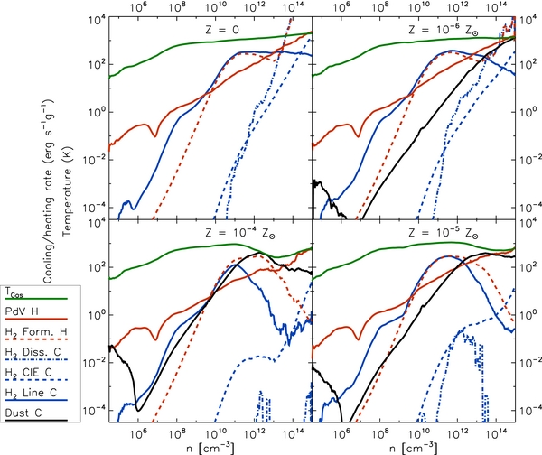
Figure 2. Cooling and heating rates vs. number density for Z = 10−4, 10−5, 10−6 Z☉, and 0. The values are calculated just before the first sink formed. The lines labeled as "C" indicate cooling, and "H" is heating. "Dust C," "H2 Line C," "H2 CIE," and "H2 Diss." indicate dust grain cooling, H2 line emission, collision-induced emission, and dissociation cooling, respectively. "H2 Form. H" and "pdV H" are the H2 formation heating rate, and compressive (pdV) heating rate.
Download figure:
Standard image High-resolution imageAt densities below n ≈ 1010 cm−3, dust cooling is unimportant in all of the runs. At these densities, the dominant coolant is H2 line emission, while the heating is dominated by compressional (pdV) heating at n ≲ 108 cm−3, and by three-body H2 formation heating at higher densities.
At higher densities, dust cooling starts to play a more important role. In the Z = 10−4 Z☉ simulation, dust cooling exceeds pdV heating at n ≈ 1010 cm−3, although it does not exceed the H2 formation heating rate until n ≈ 1011 cm−3. Once this occurs, and dust cooling dominates, the gas temperature drops sharply. In the Z = 10−5 Z☉ simulation, on the other hand, dust becomes the dominant coolant only at n ≈ 1013 cm−3, and so the temperature decrease happens later and is smaller. Finally, in the Z = 10−6 Z☉ case, dust cooling becomes competitive with pdV heating only at the very end of the simulation, and so the effect on temperature evolution is less evident.
The other thermal processes play a minor role during the collapse. For example, H2 dissociation cooling only becomes important in the runs with Z = 10−6 Z☉ and 0, and only for n > 1013 cm−3. At very high densities (n > 1014 cm−3), H2 collision-induced emission (CIE) cooling also begins to be important. For more details on H2 heating and cooling processes in this very high density regime, we refer to Clark et al. (2011a).
3.3. Fragmentation
The angular momentum is transported to smaller scales during the collapse. This process leads to the formation of a rotation supported disk-like structure. However, the rotation is not sufficient to hold the collapse of the disk, and finally it fragments forming multiple objects.
In Figure 3, we show the density structure of the gas. These snapshots were taken immediately before the first protostar was formed. Observe that at large scales the gas cloud properties are the same for all metallicities. Differences in the thermodynamic evolution appear only at n ≳ 1011 cm−3 (see Figure 1). As a consequence, we observe variations in the cloud structure only in the high-density regions.
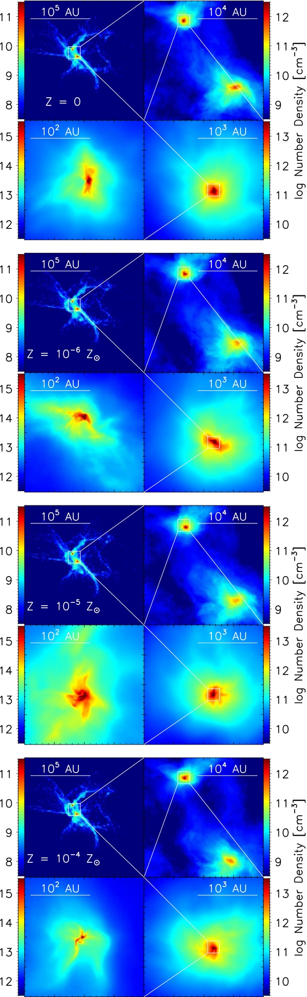
Figure 3. Number density maps for a slice through the high-density region for Z = 10−4 Z☉ (top), 10−5 Z☉, 10−6 Z☉, and 0 (bottom). The image shows a sequence of zooms in on the density structure in the gas immediately before the first protostar was formed.
Download figure:
Standard image High-resolution imageOne way to study the effect of dust cooling on the fragmentation behavior and the final stellar IMF is to look at the changes in the number of Bonnor–Ebert (MBE) masses contained in this central dense region. Using the definition from Bromm et al. (2009),

for an atomic gas with temperature T and number density n, we have computed the number of Bonnor–Ebert masses contained within a series of concentric radial spheres centered on the densest point in each of our four simulations. The results are shown in Figure 4.
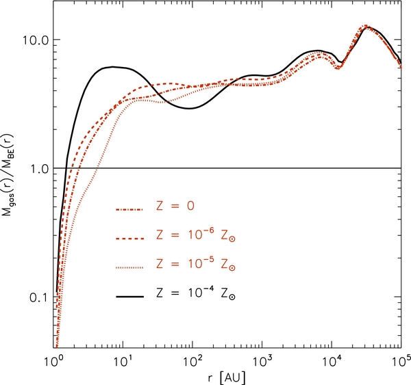
Figure 4. Enclosed gas mass divided by Bonnor–Ebert mass vs. radius for different metallicities. The values were calculated at the time just before the first sink was formed and the center is taken to be the position of the densest SPH particle.
Download figure:
Standard image High-resolution imageAt the beginning of the simulation, the cloud had ∼3 MBE. During the collapse, the gas cools and reaches ∼6 MBE in all cases. Cooling and heating are different depending on the metallicity, and this difference is seen for distances smaller than ∼400 AU. The Z = 10−4 Z☉ case, for instance, has twice the number of MBE for distances smaller than ∼10 AU, when compared to the other cases. This will have direct consequences for the fragment mass function as we will see in the next section.
When the conditions for the formation sink particle are met (see Section 2.1), such particles begin to form in the density peaks (Figure 5). Then, a disk is built up in these regions, where fragmentation also occurs (Tohline 1980). During further collapse, this dense region creates spiral structures. For Z = 10−5 Z☉ and 10−4 Z☉, density waves build up spiral structures, which become locally gravitationally unstable and go into collapse. The formation of binary systems by triple encounters (Binney & Tremaine 2008) transfers kinetic energy to some sink particles, causing them to be ejected from the high-density region. For Z = 10−5 Z☉, when the star formation efficiency (SFE) is 0.5%, fragmentation has already occurred in a secondary dense center, at a distance of ∼20 AU from the first dense region.
For Z = 10−6 Z☉ and 0, the formation of spiral structures is not observed. In these two runs, star formation occurs mainly in the central clump.
3.4. Properties of the Fragments
The simulations were stopped at a point in time when 4.7 M☉ of gas has been accreted into the sink particles. This is sufficient to identify the two fundamental modes of fragmentation discussed in Section 3.5.
Figure 6 shows the mass distribution of sink particles at that time. We typically find sink masses below 1 M☉, with somewhat smaller values in the 10−4 Z☉ case compared to the other cases. No sharp transition in fragmentation behavior was found, but rather a smooth and complex interaction between kinematic and thermodynamic properties of the cloud.
Table 1 lists the main sink particle properties. It shows that the time taken to form the first sink particle is slightly shorter for higher metallicities. This shorter time is a consequence of the more efficient cooling by dust, which decreases the thermal energy that was delaying the gravitational collapse. In Table 1 we also observe that the star formation rate is lower for Z = 10−4 Z☉. This is because star formation started at an earlier stage of the collapse, when the mean density of the cloud was lower and there was less dense gas available to form stars.
Table 1. Sink Particle Properties for the Different Metallicities at the Point where 4.7 M☉ Have Been Accreted by the Sink Particles
| Z/Z☉ | ST | FT | SFR | Mean | Median | N |
|---|---|---|---|---|---|---|
| (103 yr) | (yr) | (M☉ yr−1) | (M☉) | (M☉) | ||
| 0 | 171.6 | 73 | 0.064 | 0.24 | 0.12 | 19 |
| 10−6 | 171.2 | 72 | 0.065 | 0.29 | 0.06 | 16 |
| 10−5 | 170.8 | 88 | 0.053 | 0.24 | 0.11 | 19 |
| 10−4 | 169.2 | 138 | 0.034 | 0.10 | 0.05 | 45 |
Notes. "ST" (start time) is the time when sink particles start to form. "FT" (formation time) is the time taken to accrete 4.7 M☉ in the sinks. "SFR" is the mean star formation rate. Mean and median refer to the final mean and median sink mass. Finally, "N" is the number of sink particles formed.
Download table as: ASCIITypeset image
To better understand whether the resulting protostellar cluster was affected by varying the metallicity, we plot the final sink mass distribution in Figure 6. It shows that for the simulations with Z ⩽ 10−5 Z☉, the resulting sink particle mass function is relatively flat. There are roughly equal numbers of low-mass and high-mass stars, implying that most of the mass is to be found in the high-mass objects. This mass function is consistent with those found in other recent studies of fragmentation in metal-free gas (Greif et al. 2011; Smith et al. 2011). If the sink particle mass function provides a reliable guide to the form of the final stellar IMF, it suggests that at these metallicities, the IMF will be dominated by high-mass stars.
The resolution limit in the simulations is 2.5 × 10⁻³ M☉. All sink particles mass function presented in Figure 6 have their masses well above this value by construction. These simulations were intended to study the influence of the metallicity on the mode of star formation. Such a goal could be achieved when the sink particles have accreted a total of approximately 5 M☉. However, these systems should not be taken as star formation is completed, since the sink particles would continue accreting. Other mechanisms should also influence the mass function, and we list them in Section 4.
3.5. Timescales and Star Formation Mode
One way to explain the final mass distribution of the fragments is to look at the timescales for mass accretion and fragmentation. The degree of gravitational instability inside a volume can be represented by the number of Bonnor–Ebert masses contained in this volume. We can therefore estimate the fragmentation timescale by computing the time taken for the central dense region to accrete one Bonnor–Ebert mass. In other words, we have  , where
  is the accretion rate. This value is shown as a function of the enclosed gas mass in Figure 7, where the values are calculated for particles in spherical shells, and the center is taken to be the densest SPH particle.
  is obtained by summing up the mass of the particles (mp) inside a shell times their radial velocity (vr),
  . This way of estimating the expected mass accretion in the sink particles is motivated by the results in Clark et al. (2011b, see their Figure 3(b)). They demonstrate that the mass accretion rate based on the radial mass infall profile is a good estimate of that actually measured by the sink particles.
For comparison, we also plot the accretion timescale, here defined as the time taken by the gas to accrete the mass enclosed by that radius,  . When the fraction tfrag/tacc > 1, one expects that the gas enclosed by this shell is going to be accreted faster than it can fragment, favoring high-mass objects. Conversely, for tfrag/tacc < 1, the gas will fragment faster than it can be accreted by the existing fragments, and the final mass distribution is expected to have more low-mass objects. Note that as defined here, the timescale on which new fragments form tfrag/tacc is the inverse of the quantity Mgas/MBE plotted in Figure 4.
In Figure 7, the simulation with Z = 10−4 Z☉ has the lowest values for tfrag/tacc, over a wide range of Menc. This indicates that more low-mass fragments are expected to form in this case, leading to a steeper fragment mass function.
Now we can compare the predicted values before sink formation started with the final accretion and fragmentation timescales. These values are designed to represent the characteristic timescales on which the mass histogram changes: the fragmentation timescale (τfrag) is the time in which the number of fragments change by a significant amount, while the accretion timescale (τacc) represents the time in which the existing fragments grow in mass. We therefore define  , and
, and  , where n is the number of sink particles and M is the total mass incorporated into sink particles.
Both timescales should increase over time, since the number of sink particles and the total mass also increase. This reflects the fact that it takes longer to change the shape of the mass histogram in frequency when the number of elements is higher, and in mass when the total mass is high. The key point is that these timescales are related to the shape of the histogram. If the timescale for accretion is shorter than the timescale for fragmentation, the histogram will tend to be dominated by high-mass objects. Conversely, if the fragmentation timescale is shorter than the accretion timescale, the low-mass part will be populated before the objects can grow and occupy higher mass bins. Therefore, a comparison between τacc and τfrag helps us to understand the shape of the mass histogram.
We calculate the average τacc and τfrag at each point in time. The value for the mean τfrag and τacc is calculated by the time-weighted individual times as in Equations (2) and (3):


where i refers to each snapshot of the simulation, and it varies from two to the total number of snapshots. ni, Mi, ti, and t are the number of sink particles, the total mass in sinks, the time at the snapshot i, and the total time of sink particle formation in each simulation, respectively. 〈M〉 is the average mass of a sink particle in the simulations including all metallicities. This average mass (〈M〉) is used to make τacc in units of time, and comparable to the accretion time. Other values were tried, such as the total average mass for each metallicity. However, the accretion time was not affected considerably. Thus, the comparison between accretion and fragmentation leads to qualitatively equal results, independent of the value used to get the correct dimension for τacc.
Important to note that τfrag, merging is calculated in the same way as τfrag, with the difference that the number of sink particles (ni) is always lower or equal to the non-merging case. That is why τfrag, merging has higher values when compared to τfrag.
Figure 8 shows the average timescales for fragmentation and accretion for different metallicities. We also plot the values considering the sink particles that could have merged due to collisions (see Section 4). These results explain the difference in the sink particle mass distribution in Figure 6. For Z ⩽ 10−5 Z☉, the fragmentation time is always larger than the accretion time, indicating that the sink particles will accrete faster than they can be generated, resulting in a flatter mass distribution. On the other hand, when the fragmentation time is longer than the accretion time (for Z = 10−4 Z☉), the gas fragments, rather than moving to the center and being accreted. As a consequence, the low-mass end of the protostellar mass function grows faster than the high-mass end, and the slope of the mass function steepens. This behavior agrees well with the predictions from before fragmentation started, as shown in Figure 7.
Note that the values in Figure 7 were calculated before the formation of the first sink particle, while the values in Figure 8 were calculated using the sink particle properties. A comparison between them is useful to evaluate whether the gas cloud properties from before star formation started could be used to predict its star formation behavior. The trend in both figures is that the fragmentation timescale is normally shorter than the accretion timescales for Z = 10−4 Z☉. From these results we conclude that the mass distribution in Figure 6 can be explained by the timescales in Figure 8, in particular the fact that the Z ⩽ 10−5 Z☉ simulations have more high-mass objects. The last finding is that the transition from Pop III to Pop II star formation mode is not abrupt, in the sense that there is no metallicity below which the gas cannot fragment. The transition is rather in the stellar IMF, and gas clouds with Z ≲ 10−5 Z☉ form a more flat IMF, while gas clouds with Z ≳ 10−4 Z☉ produce a cluster with more low-mass objects (see also Clark et al. 2008).
3.6. Radial Mass Distribution
Another property of the star-forming cloud that we observed to vary in our calculations is the spatial mass distribution. The dependence of the enclosed gas and sink mass on the distance from the center of mass is shown in Figure 9. The Z = 0 case has almost all of the sink particle mass concentrated within r < 8 AU. The gas density for this case is also higher in this region, when compared to the other metallicities, showing that the gas and sink particle mass densities follow each other. The mass in sink particles exceeds the gas mass for small radii, being the most important component in the gravitational potential. For r > 150 AU, the gas becomes the most massive component, for all Z. Girichidis et al. (2012) also reported this behavior, but in their case the sink particles already started to dominate the potential below r ≈ 103 AU.
This higher concentration of gas and sinks at the center occurs because for the Z = 0 case, the gas had higher temperatures in the central region. For high temperatures, the criterion for gravitational instability requires higher densities, which are achieved only very close to the center. As a consequence, the sink particle formation criteria are met just for short distances from the center.
Consequently, the dominance of sink particles mass in the gravitational potential over the gas mass, for radii smaller than 150 AU, shows the importance of treating gas and stars together in this sort of problem. It also suggests that N-body effects, such as ejections and close encounters, should play an important role in the formation of these dense star clusters, even in the very earliest stages of their evolution (see Smith et al. 2011; Greif et al. 2012).
4. CAVEATS
Our aim with these calculations is to study the importance of dust cooling for fragmentation in high-redshift halos. To better understand star formation in this environment, additional physical processes should be considered as well.
Particularly, the low number of sink particles (≈20) and the small SFE (0.5%) do not permit us to constrain the stellar IMF adequately. By running the calculations until the SFE goes toward higher values, uncertainties involving the fragments that formed during the simulations can be diminished. However, this does not appear to be computationally feasible with our current approach.
The mass accreted by the sink particles varies with the different metallicities, and affects the final sink particle mass function. It also influences the expected accretion luminosity. We did not take this process into account during our calculations, but we can estimate its importance relative to other thermal processes.
In Figure 10 we present the accretion properties for the newborn stellar systems. The top panel shows how the total mass in sinks evolves with time, for different metallicities. The accretion rate varies from 0.02 to 0.17 M☉ yr−1, and it is on average lower for the Z = 10−4 Z☉ case.
In the bottom panel of Figure 10, we show the accretion luminosity calculated by adding up all sink particle contributions, with the standard equation,

where  is the mass accretion rate by a protostar with mass M*, and stellar radius R*. We calculate R* following Stahler et al. (1986) using

The accretion luminosity varies from a few times 103 L☉ to around 50 × 103 L☉, depending on metallicity. For Z ⩽ 10−5 Z☉, the accretion luminosity is always over 104 L☉. The Z = 10−4 Z☉ case has the lowest estimated accretion luminosity, around four times lower than the other cases. The values found for the accretion luminosity are similar to the ones found by Smith et al. (2011) for Z = 0, where they argue that accretion luminosity could delay the fragmentation, but not prevent it.
We can now compare this expected luminosity, and its consequent heating, to the heating processes in Figure 2. We make the assumption that gas and dust are absorbing the radiation in the optically thin regime. This overestimates the effects, and we obtain an upper limit for the accretion luminosity heating,

where ρg is the gas density, κP is the Planck mean opacity, and r is the distance from the source. We also assume that heating occurs at ρ ≈ 10−9 g cm−3. With this assumption we can calculate the mean gas temperature, and use the Planck mean opacity for the gas from Mayer & Duschl (2005), for their fiducial Pop III chemical composition. The Planck mean opacity for the dust is calculated in the same way as in Dopcke et al. (2011). Finally, the combined Planck mean opacity is the sum of gas and dust contributions, κP ≡ κgas + κdust.
By considering the maximum accretion luminosity for each case, we obtain that Γacc = 4.9, 0.9, 1.7, and  , for Z = 10−4, 10−5, 10−6, and 0 Z☉.
As these values are comparable to the other thermal processes at high densities (see Figure 2), it would seem that accretion luminosity heating from the young protostars may have some effect on the way in the which the gas behaves. However without doing the radiative transfer explicitly, it is difficult to estimate how big this effect will be.
Although the amount of heating seems high, the dust cooling is a strong function of temperature in this regime, and so it could be that dust temperatures remain quite similar. One must also remember that the above estimates do not take into account the extinction and reprocessing of the radiation field that will occur in the optically thick region that surrounds the protostar. However, even a factor-of-two change in the dust temperature will remove the dip in the ρ − T phase diagrams that we show in Figure 1, and thus remove the ability of the dust to set a new length scale for fragmentation.
Sufficiently far enough away from the strongest sources, the effect will obviously drop to the point at which the physics in our current calculations are applicable. However if we look to Figure 5, we see that most of the fragmentation that we report is confined to a few tens of AU around the central protostar, and as such, the effects of the accretion luminosity are likely to change the picture that we present in this paper to some extent. We hope to explore this effect in a future study.
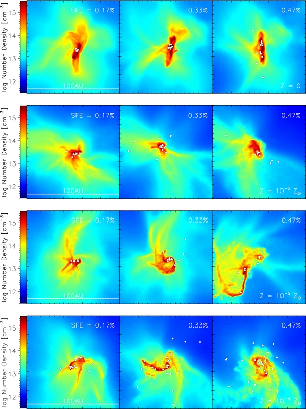
Figure 5. Number density map showing a slice through the densest clump, and the star formation efficiency (SFE) for Z = 10−4 Z☉ (bottom), 10−5 Z☉, 10−6 Z☉, and 0 (top). The box is 100 AU × 100 AU and the percentage indicates the star formation efficiency, i.e., the total mass in the sinks divided by the cloud mass (1000 M☉).
Download figure:
Standard image High-resolution imageAnother aspect of our model that could be improved upon are the dust opacities. The thermal evolution can be calculated more accurately if we use dust opacities that better represent the values expected for very low metallicity environments. The dust opacity in our simulations corresponds to values calculated for the Milky Way and then scaled with metallicity. This means that the opacity values for the Z = 10−4 Z☉ case are 10−4 times the dust opacity in the Milky Way. This approximation is probably not fully correct, and the use of a more accurate model (e.g., Todini & Ferrara 2001; Bianchi & Schneider 2007; Schneider et al. 2012; Nozawa et al. 2003, 2006) can change the value of the cooling in the region where fragmentation occurs. This change affects the local Jeans mass, and consequently the star formation behavior.
Furthermore, the available models give the dust composition for different scenarios in the early universe, e.g., different supernovae progenitor masses (Schneider et al. 2012), and the use of such models would add another variable to the problem—the stellar population for the supernovae progenitors. One reasonable approach is to test different scenarios and see how they would affect the properties of the cluster of stars that forms. In this sense, the dust composition is a problem in itself that should be addressed. Since cooling affects the fragmentation behavior and mass accretion, a more realistic dust model improves the accuracy with which we can model star formation at low metallicities. We intend to address this issue in a future paper.
Another effect that could change our results is the possibility of inelastic encounters between the protostars. Star formation in our simulation occurs at very high densities, where inelastic encounters between the new born protostars could occur. In similar conditions to the ones tested here, Smith et al. (2011, 2012) show that the estimated stellar radius could be as large as ∼1 AU, a value comparable to the distances between the sink particles shown in Figure 5. By not accounting for merging of such objects, we could be overestimating the final number of fragments, although we expect new protostars to continue to form.
Since collisions may result in merging, we estimated this effect by comparing the sink particle distances and estimated radii. The stellar radii were calculated following Equation (5). By considering that every collision resulted in merging, we concluded that the number of merged objects is relatively the same for all simulations (see Table 2). Also when we compare the mode of star formation, the discrepancy on the mode of star formation for the Z = 10−4 Z☉ only becomes more evident. The particles that collided have most often masses higher than 0.1 M☉, therefore the low-mass part of Figure 6 had not changed considerably. This means that the conclusions about the mode of star formation in Section 3.5 are not strongly affected by merging. The simulation with Z = 10−4 Z☉ remains with a more present-day-like stellar mass distribution, even when merging is considered.
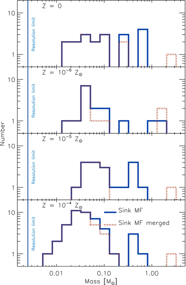
Figure 6. Sink particle mass function at the point when 4.7 M☉ of gas had been accreted by the sink particles. The mass resolution of the simulations is indicated by the vertical line. We also plot the sink mass function considering the sink particles that could have merged due to collisions (see Section 4).
Download figure:
Standard image High-resolution image
Figure 7. Timescales for fragmentation (top panel) and accretion (middle panel), and also their ratio (bottom panel) according to the radius for the metallicities tested. The values were calculated just before the first sink particle was formed.
Download figure:
Standard image High-resolution imageTable 2. Sink Particle Properties Considering That All Collisions Resulted on Merging
| Z/Z☉ | Nam | Nmerged | Mean | Coll. Mean |
|---|---|---|---|---|
| (M☉ yr−1) | (M☉ yr−1) | |||
| 0 | 14 | 5 | 0.34 | 0.65 |
| 10−6 | 11 | 5 | 0.43 | 0.81 |
| 10−5 | 12 | 7 | 0.39 | 0.53 |
| 10−4 | 38 | 7 | 0.13 | 0.38 |
Notes. "Nam" is the remaining number of sink particles after merging, "Nmerged is the number of those that could have merged. Note that Nam + Nmerged recovers the number of sink particles (N) in Table 1. "Mean" refers to the new mean sink particle mass and "Coll. Mean" refers to the mean mass of the particles that collided.
Download table as: ASCIITypeset image
Also in Figure 8 we show the fragmentation time, when merging is considered. The important fact that the fragmentation time is shorter than the accretion timescale for Z = 10−4 Z☉ is not affected by merging. The noticeable change is that the ratio τfrag/τacc becomes shorter for the simulation with Z = 0. This means that for this case, the overall fragmentation is inhibited, and more high-mass objects will form.
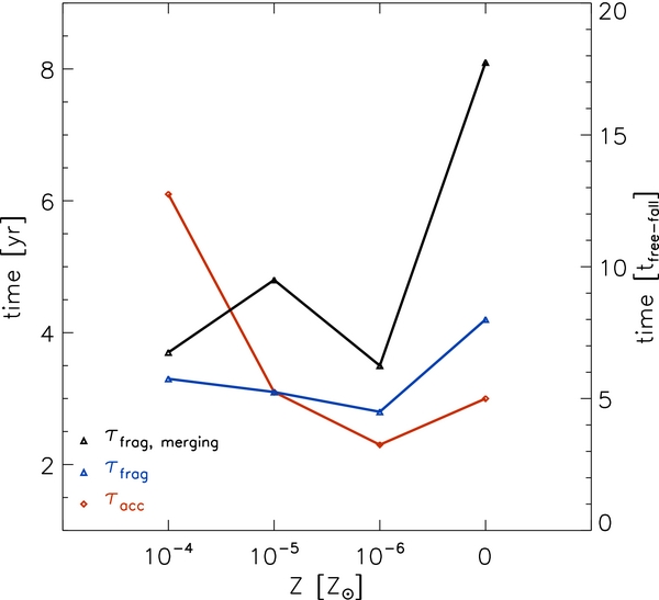
Figure 8. Timescales for fragmentation and accretion for different metallicities calculated for the sink particles following Equations (2) and (3). τfrag, merged refers to the values considering that sink particles can merge due to collisions (see Section 4).
Download figure:
Standard image High-resolution image
Figure 9. Dependence of the enclosed gas and sink mass on the distance from the center of mass, for the four simulations. The values were calculated at a point when 4.7 M☉ of gas had been accreted.
Download figure:
Standard image High-resolution image
Figure 10. Time evolution of the mass, mass accretion rate, and accretion luminosity for the four metallicities, for all sink particles combined.
Download figure:
Standard image High-resolution image
Finally, the inclusion of magnetic fields in the calculations could alter the fragmentation picture as it is presented in this study. They can be amplified during gravitational collapse (Schleicher et al. 2010), generating values strong enough to delay the collapse (Schleicher et al. 2009; Sur et al. 2010; Federrath et al. 2011a, 2011b; Turk et al. 2012). Analytic amplification values are calculated by Schober et al. (2012). From modeling present-day star formation, we know that the presence of magnetic fields can decrease the level of fragmentation, but cannot prevent it, for the expected saturation levels of a few percent (Peters et al. 2011; Hennebelle et al. 2011).
5. CONCLUSIONS
In this paper we have studied the physical mechanism involved in the fragmentation of star-forming gas clouds in the early universe. We run a set of four hydrodynamic simulations with metallicities varying from the metal-free case to Z = 10−4 Z☉. To model the thermodynamic evolution, we included a chemical network for metal-free gas, with the addition of dust cooling.
As a result, we found that dust can cool the gas for number densities higher than 1011, 1012, and 3 × 1013 cm−3 for Z = 10−4, 10−5, and 10−6 Z☉, respectively. Higher metallicity implies larger dust-to-gas fraction, and consequently stronger cooling. This is reflected in a lower temperature of the dense gas for the higher metallicity simulations, and this colder gas permitted a faster collapse. Therefore, the fragmentation behavior of the gas depends on the metallicity, and higher metallicities lead to a faster collapse.
For example, the characteristic fragment mass was lower for Z = 10−4 Z☉, since a lower temperature reduces the Bonnor–Ebert masses at the point where the gas undergoes fragmentation. This also implies a lower ratio of fragmentation and accretion time, tfrag/tacc, which will lead to a mass function dominated by low-mass objects. For Z ⩽ 10−5 Z☉, fragmentation and accretion timescales are comparable, and the resulting mass spectrum is rather flat, with roughly equal numbers of stars in each mass bin.
In addition to that, dust cooling appears to be insufficient to change the stellar mass distribution for the Z = 10−5 and 10−6 Z☉ cases, when compared with the metal-free case. This can be seen in the sink particle mass function (Figure 6), which shows that the Z ⩽ 10−5 Z☉ cases do not appear to be fundamentally different.
Finally, we conclude that the dust is not an efficient coolant at metallicities below or equal to Zcrit = 10−5 Z☉, in the sense that it cannot change the fragmentation behavior for these metallicities. Our results support the idea that low-mass fragments can form in the absence of metals, and clouds with Z ≲ Zcrit will form a cluster with a flat IMF.
We thank Tom Abel, Volker Bromm, Kazuyuki Omukai, Raffaella Schneider, Rowan Smith, and Naoki Yoshida for useful comments. The present work is supported by contract research "Internationale Spitzenforschung II" of the Baden-Württemberg Stiftung (grant P-LS-SPII/18), the German Bundesministerium für Bildung und Forschung via the ASTRONET project STAR FORMAT (grant 05A09VHA), a Frontier grant of Heidelberg University sponsored by the German Excellence Initiative, the International Max Planck Research School for Astronomy, and Cosmic Physics at the University of Heidelberg (IMPRS-HD). All computations described here were performed at the Leibniz-Rechenzentrum, National Supercomputer HLRB-II (Bayerische Akademie der Wissenschaften), on the HPC-GPU Cluster Kolob (University of Heidelberg), and on the Ranger cluster at the Texas Advanced Computing Center, as part of project TG-MCA995024.