


ABSTRACT
We present a new N-body and gas dynamics code, called Nyx, for large-scale cosmological simulations. Nyx follows the temporal evolution of a system of discrete dark matter particles gravitationally coupled to an inviscid ideal fluid in an expanding universe. The gas is advanced in an Eulerian framework with block-structured adaptive mesh refinement; a particle-mesh scheme using the same grid hierarchy is used to solve for self-gravity and advance the particles. Computational results demonstrating the validation of Nyx on standard cosmological test problems, and the scaling behavior of Nyx to 50,000 cores, are presented.
Export citation and abstract BibTeX RIS
1. INTRODUCTION
Understanding how the distribution of matter in the universe evolves throughout cosmic history is one of the major goals of cosmology. Properties of the large-scale structure depend strongly on a cosmological model, as well as the initial conditions in that model. Thus, in principle, we can determine the cosmological parameters of our universe by matching the observed distribution of matter to the best-fit calculated model universe. This is much easier said then done. Observations, with the exception of gravitational lensing, cannot directly access the dominant form of matter, the dark matter. Instead they reveal information about baryons, which in some biased way trace the dark matter. On the theory side, equations describing the evolution of density perturbations (e.g., Peebles 1980) can be easily solved only when the amplitude of perturbations is small. However, in most systems of interest, the local matter density, ρ, can be several orders of magnitude greater than the average density, ρ0, making the density contrast, δ ≡ (ρ − ρ0)/ρ0, much greater then unity.
Due to this nonlinearity, and the uncertainty in the initial conditions of the universe, a single "heroic" simulation is not sufficient to resolve most of the cosmological questions of interest; the ability to run many simulations of different cosmologies, with different approximations to the governing physics, is imperative. Semi-analytic models (for example, White & Frenk 1991 in the context of galaxy formation) or scaling relations (e.g., Smith et al. 2003) present an interesting alternative to expensive simulations, but they must also be validated or calibrated by simulations in order to be trustworthy. Finally, besides being an invaluable theorist's tool, simulations play a crucial role in bridging the gap between theory and observation, something that is becoming more and more important as large sky surveys are starting to collect data.
To match the capabilities of future galaxy/cluster surveys, cosmological simulations must be able to simulate volumes ∼1 Gpc on a side while resolving scales on the order of ∼10 kpc or even smaller. Clearly, in the context of Eulerian gas dynamics, this requires the ability to run simulations with multiple levels of refinement that follow the formation of relevant objects. To resolve L* galaxies with ∼100 mass elements (particles) per galaxy in simulations of this scale, one needs tens of billions of particles. Such systems, with crossing times of a million years or less, must be evolved for ∼10 billion years. On the other side of the spectrum are simulations aimed at predicting Lyα forest observations, where the dynamical range is more like ∼104, but as most of the contribution from the forest comes from gas at close to mean density, most of the computational volume must be resolved. These simulations require much "shallower" mesh refinement strategies covering a larger fraction of the domain.
In addition to the challenge of achieving sufficient refinement, simulations need to incorporate a range of different physics beyond the obvious self-gravity. The presence of baryons introduces corrections to gravity-only predictions; these corrections are negligible at very large scales, but become increasingly significant at smaller scales, requiring an accurate treatment of the gas in order to provide realistic results that can be directly compared to observations. Radiative cooling and heating mechanisms are as influential on many observables as the addition of the gas itself, but large uncertainties remain in these terms, and our lack of knowledge increases as we move into highly nonlinear systems. Thus, we can model low density Lyα absorbers at higher redshift (e.g., Viel et al. 2005), we can reproduce the bulk properties of the biggest objects in the universe—galaxy clusters (see, e.g., Stanek et al. 2010), but on smaller and much denser scales galaxy formation still remains elusive and is a field of active research (e.g., Benson 2010).
In this paper, we present a newly developed N-body and gas dynamics code called Nyx. The code models dark matter as a system of Lagrangian fluid elements, or "particles," gravitationally coupled to an inviscid ideal fluid representing baryonic matter. The fluid is modeled using a finite volume representation in an Eulerian framework with block-structured adaptive mesh refinement (AMR). The mesh structure used to evolve fluid quantities is also used to evolve the particles via a particle-mesh (PM) method. In order to more accurately treat hypersonic motions, where the kinetic energy is many orders of magnitude larger than the internal energy of the gas, we employ the dual energy formulation, where both the internal and total energy equations are solved on the grid during each time step.
There are a number of existing finite volume, AMR codes; most commonly used in the cosmology community are Enzo (Bryan et al. 1995), ART (Kravtsov et al. 1997), FLASH (Fryxell et al. 2000), and RAMSES (Teyssier 2002). Enzo, FLASH, and Nyx are all similar in that they use block-structured AMR; RAMSES and ART, by contrast, refine locally on individual cells, resulting in very different refinement patterns and data structures. Among the block-structured AMR codes, Enzo and FLASH enforce a strict parent-child relationship between patches; i.e., each refined patch is fully contained within a single parent patch. FLASH also enforces that all grid patches have the same size. Nyx requires only that the union of fine patches be contained within the union of coarser patches with suitable proper nesting. Again, this results in different refinement patterns, data structures, communication overhead, and scaling behavior.
Time-refinement strategies vary as well. FLASH advances the solution at every level with the same time step, Δt, while Enzo, ART and RAMSES allow for subcycling in time. A standard subcycling strategy enforces that Δt/Δx is constant across levels; ART and Enzo allow greater refinement in time than space when appropriate. Nyx maintains several different subcycling strategies. The user can specify at run-time that Nyx use no subcycling, standard subcycling, a specified subcycling pattern or "optimal subcycling." In the case of optimal subcycling, Nyx chooses, at specified coarse time intervals during a run, the most efficient subcycling pattern across all levels based on an automated assessment of the computational cost of each option at that time (E. Van Andel et al. 2013, in preparation).
One of the major goals behind the development of a new simulation code, in an already mature field such as computational cosmology, is to ensure effective utilization of existing and future hardware. Future large-scale cosmological simulations will require codes capable of efficient scaling to hundreds of thousands of cores, and effective utilization of the multicore, shared memory, nature of individual nodes. One such code for gravity-only simulations is HACC (Habib et al. 2009). The frameworks for existing hydro codes such as Enzo and FLASH are currently being substantially rewritten for current and future architectures. Nyx, like the CASTRO code for radiation-hydrodynamics (Almgren et al. 2010; Zhang et al. 2011), and the MAESTRO code for low Mach number astrophysics (Almgren et al. 2006a, 2006b; Almgren et al. 2008; Zingale et al. 2009; Nonaka et al. 2010), is built on the BoxLib (BoxLib 2011) software framework for block-structured adaptive mesh methods, and as such it leverages extensive efforts to achieve the massively parallel performance that future simulations will demand. BoxLib currently supports a hierarchical programming approach for multicore architectures based on both MPI and OpenMP. Individual routines, such as those to evaluate heating and cooling source terms, are written in a modular fashion that makes them easily portable to GPUs.
In the next section we present the equations that are solved in Nyx. In Section 3 we present an overview of the code, and in Section 4 we discuss structured grid AMR and the multilevel algorithm. Section 5 describes in more detail the parallel implementation, efficiency and scaling results. Section 6 contains two different cosmological tests; the first is a pure N-body simulation, and the second is the Santa Barbara cluster simulation, which incorporates both gas dynamics and dark matter. In the final section we discuss future algorithmic developments and upcoming simulations using Nyx.
2. BASIC EQUATIONS
2.1. Expanding Universe
In cosmological simulations, baryonic matter is evolved by solving the equations of self-gravitating gas dynamics in a coordinate system that is comoving with the expanding universe. This introduces the scale factor, a, into the standard hyperbolic conservation laws for gas dynamics, where a is related to the redshift, z, by a = 1/(1 + z), and can also serve as a time variable. The evolution of a in Nyx is described by the Friedmann equation that, for the two-component model we consider, with Hubble constant, H0, and cosmological constant,  , has the form

where Ω0 is the total matter content of the universe today.
2.2. Gas Dynamics
In the comoving frame, we relate the comoving baryonic density, ρb, to the proper density, ρproper, by ρb = a3ρproper, and define U to be the peculiar proper baryonic velocity. The continuity equation is then written as

Keeping the equations in conservation form as much as possible, we can write the momentum equation as

where the pressure, p, is related to the proper pressure, pproper, by p = a3pproper. Here g = −∇ϕ is the gravitational acceleration vector.
We use a dual energy formulation similar to that used in Enzo (Bryan et al. 1995), in which we evolve the internal energy as well as the total energy during each time step. The evolution equations for internal energy, e, and total energy, E = e + (1/2)U2, can be written:


where ΛHC represents the combined heating and cooling terms. We synchronize E and e at the end of each time step; the procedure depends on the magnitude of e relative to E, and is described in the next section.
We consider the baryonic matter to satisfy a gamma-law equation of state (EOS), where we compute the pressure, p = (γ − 1)ρe, with γ = 5/3. The composition is assumed to be a mixture of hydrogen and helium in their primordial abundances with the different ionization states for each element computed by assuming statistical equilibrium. The details of the EOS and how it is related to the heating and cooling terms will be discussed in future work. Given γ = 5/3, we can simplify the energy equations to the form


2.3. Dark Matter
Matter content in the universe is strongly (80–90%) dominated by cold dark matter, which can be modeled as a non-relativistic, pressureless fluid. The evolution of the phase-space function, f, of the dark matter is thus given by the collisionless Boltzmann (aka Vlasov) equation, which in expanding space is

where m and p are mass and momentum, respectively, and ϕ is the gravitational potential.
Rather than trying to solve Vlasov equation directly, we use Monte Carlo sampling of the phase-space distribution at some initial time to define a particle representation, and then evolve the particles as an N-body system. Since particle orbits are integrals of a Hamiltonian, Liouville's theorem ensures that at some later time particles are still sampling the phase space distribution as given in Equation (8). Thus, in our simulations we represent dark matter as discrete particles with particle i having comoving location, xi, and peculiar proper velocity, ui, and solve the system


where gi is gravitational acceleration evaluated at the location of particle i, i.e., gi = g(xi, t).
2.4. Self-gravity
The dark matter and baryons both contribute to the gravitational field and are accelerated by it. Given the comoving dark matter density, ρdm, we define ϕ by solving

where G is the gravitational constant and ρ0 is the average value of (ρdm + ρb) over the domain.
3. CODE OVERVIEW
3.1. Expanding Universe
Before evolving the gas and dark matter forward in time, we compute the evolution of a over the next full coarse level time step. Given an defined as a at time tn, we calculate an + 1 via m second-order Runge–Kutta steps. The value of m is chosen such that the relative difference between an + 1 computed with m and 2m steps is less than 10−8. This accuracy is typically achieved with m = 8–32, and the computational cost of advancing a is trivial relative to other parts of the simulation. We note that Δt is constrained by the growth rate of a such that a changes by no more than 1% in each time step at the coarsest level. Once an + 1 is computed, values of a needed at intermediate times are computed by linear interpolation between an and an + 1.
3.2. Gas Dynamics
We describe the state of the gas as U = (ρb, aρbU, a2ρbE, a2ρbe), then write the evolution of the gas as

where F = (1/a ρbU, ρbUU, a(ρbUE + pU), aρbUe) is the flux vector, Se = (0, 0, 0, −ap∇ · U) represents the additional term in the evolution equation for internal energy, Sg = (0, ρbg, aρbU · g, 0) represents the gravitational source terms, and SHC = (0, 0, aΛHC, aΛHC) represents the combined heating and cooling source terms. The state, U, and all source terms are defined at cell centers; the fluxes are defined on cell faces.
We compute F using an unsplit Godunov method with characteristic tracing and full corner coupling (Colella 1990; Saltzman 1994). See Almgren et al. (2010) for a complete description of the algorithm without the scale factor, a; here we include a in all terms as appropriate in a manner that preserves second-order temporal accuracy. The hydrodynamic integration supports both unsplit piecewise linear (Colella 1990; Saltzman 1994) and unsplit piecewise parabolic method (PPM) schemes (Miller & Colella 2002) to construct the time-centered edge states used to define the fluxes. The piecewise linear version of the implementation includes the option to include a reference state, as discussed in Colella & Woodward (1984) and Colella & Glaz (1985). We choose as a reference state the average of the reconstructed profile over the domain of dependence of the fastest characteristic in the cell propagating toward the interface. (The value of the reconstructed profile at the edge is used if the fastest characteristic propagates away from the edge.) This choice of reference state minimizes the degree to which the algorithm relies on the linearized equations. In particular, this choice eliminates one component of the characteristic extrapolation to edges used in second-order Godunov algorithms. For the hypersonic flows typical of cosmological simulations, we have found the use of reference states improves the overall robustness of the algorithm. The Riemann solver in Nyx iteratively solves the Riemann problem using a two-shock approximation as described in Colella & Glaz (1985); this has been found to be more robust for hypersonic cosmological flows than the simpler linearized approximate Riemann solver described in Almgren et al. (2010). In cells where e is less than 0.01% of E, we use e as evolved independently to compute temperature and pressure from the EOS and redefine E as e + (1/2)U2; otherwise we redefine e as E − (1/2U2).
The gravitational source terms, Sg, in the momentum and energy equations are discretized in time using a predictor-corrector approach. Two alternatives are available for the discretization of ρbU · g in the total energy equation. The most obvious discretization is to compute the product of the cell-centered momentum, (ρbU), and cell-centered gravitational vector, g, at each time. While this is spatially and temporally second-order accurate, it can have the un-physical consequence of changing the internal energy, e = E − (1/2)U2, since the update to E is analytically but not numerically equivalent to the update to the kinetic energy calculated using the updates to the momenta. A second alternative defines the update to E as the update to (1/2)U2. A more complete review of the design choices for including self-gravity in the Euler equations is given in Springel (2010).
3.3. Dark Matter
We evolve the positions and velocities of the dark matter particles using a standard kick-drift-kick sequence, identical to that described in, for example, Miniati & Colella (2007). We compute gi at the ith particle's location, xi by linearly interpolating g from cell centers to xi. To move the particles, we first accelerate the particle by Δt/2, then advance the location using this time-centered velocity:


After gravity has been computed at time tn + 1, we complete the update of the particle velocities,

We observe that this scheme is symplectic, thus conserves the integral of motion on average (Yoshida 1993). Computationally the scheme is also appealing because no additional storage is required during the time step to hold intermediate positions or velocities.
3.4. Self-gravity
We define ρdm on the mesh using the cloud-in-cell scheme, whereby we assume the mass of the ith particle is uniformly distributed over a cube of side Δx centered at xi. We assign the mass of each particle to the cells on the grid in proportion to the volume of the intersection of each cell with the particle's cube, and divide these cell values by Δx3 to define the comoving density that contributes to the right-hand side of Equation (11).
We solve for ϕ on the same cell centers where ρb and ρdm are defined. The Laplace operator is discretized using the standard seven-point finite difference stencil and the resulting linear system is solved using geometric multigrid techniques, specifically V-cycles with red-black Gauss–Seidel relaxation. The tolerance of the solver is typically set to 10−12, although numerical exploration indicates that this tolerance can be relaxed. While the multigrid solvers in BoxLib support Dirichlet, Neumann, and periodic boundary conditions, for the cosmological applications presented here we always assume periodic boundaries. Further gains in efficiency result from using the solution from the previous Poisson solve as an initial guess for the new solve.
Given ϕ at cell centers, we compute the average value of g over the cell as the centered difference of ϕ between adjacent cell centers. This discretization, in combination with the interpolation of g from cell centers to particle locations described above, ensures that on a uniform mesh the gravitational force of a particle on itself is identically zero (Hockney & Eastwood 1981).
3.5. Computing the Time Step
The time step is computed using the standard CFL condition for explicit methods, with additional constraints from the dark matter particles and from the evolution of a. Using the user-specified hyperbolic CFL factor, 0 < σCFL, hyp < 1, and the sound speed, c, computed by the EOS, we define

where ei is the unit vector in the ith direction and max x is the maximum taken over all computational grid cells in the domain.
The time step constraint due to particles requires that the particles not move farther than Δx in a single time step. Since un + 1/2i is not yet known when we compute the time step, Δt at time tn, for the purposes of computing Δt, we estimate un + 1/2i by uni. Using the user-specified CFL number for dark matter, 0 < σCFL, dm < 1, which is independent of the hyperbolic CFL number, we define

where max j is the maximum taken over all particles j. The default value for σCFL, dm = 0.5. In cases where the particle velocities are initially small but the gravitational acceleration is large, we also constrain Δtdm by requiring that giΔt2dm < Δx for all particles to prevent rapid acceleration resulting in a particle moving too far.
Finally, we compute Δta as the time step over which a would change by 1%. The time step taken by the code is set by the smallest of the three:

We note that non-zero source terms can also potentially constrain the time step; we defer the details of that discussion to a future paper.
3.6. Single-level Integration Algorithm
The algorithm at a single level of refinement begins by computing the time step, Δt, and advancing a from tn to tn + 1 = tn + Δt. The rest of the time step is then composed of the following steps:
- Step 1: Compute ϕn and gn using ρnb and ρndm, where ρndm is computed from the particles at xni.We note that in the single-level algorithm we can instead use g as computed at the end of the previous step because there have been no changes to xi or ρb since then.
- Step 2: Advance U by Δt.If we are using a predictor-corrector approach for the heating and cooling source terms, then we include all source terms in the explicit update:where Fn + 1/2 and Sn + 1/2e are computed by predicting from the Un states.If we are instead using Strang splitting for the heating and cooling source terms, we first advance (ρe) and ρE by integrating the source terms in time for (1/2)Δt
 then advance the solution using time-centered fluxes and Se and an explicit representation of Sg at time tn:where Fn + 1/2 and Sn + 1/2e are computed by predicting from the Un,* states. The details of how the heating and cooling source terms are incorporated depend on the specifics of the heating and cooling mechanisms represented by ΛHC; we defer the details of that discussion to a future paper.
 - Step 3: Interpolate gn from the grid to the particle locations, then advance the particle velocities by Δt/2 and particle positions by Δt:
- Step 4: Compute ϕn + 1 and gn + 1 using ρn + 1,*b and ρn + 1dm, where ρn + 1dm is computed from the particles at xn + 1i.Here we can use ϕn as an initial guess for ϕn + 1 in order to reduce the time spent in multigrid to reach the specified tolerance.
- Step 5: Interpolate gn + 1 from the grid to the particle locations, then update the particle velocities, un + 1i
- Step 6: Correct U with time-centered source terms, and replace e by E − (1/2)U2 as appropriate.If we are using a predictor-corrector approach for the heating and cooling source terms, we correct the solution by effectively time-centering all the source terms:If we are using Strang splitting for the heating and cooling source terms, we time-center the gravitational source terms only,then integrate the source terms for another (1/2)Δt,We note here that the time discretization of the gravitational source terms differs from that in Enzo (Bryan et al. 1995), where Sn + 1/2g is computed by extrapolation from values at tn and tn − 1.If, at the end of the time step, (ρE)n + 1 − (1/2)ρn + 1(Un + 1)2 > 10−4(ρE)n + 1, we redefine (ρe)n + 1 = (ρE)n + 1 − (1/2)ρn + 1(Un + 1)2; otherwise we use en + 1 as evolved above when needed to compute pressure or temperature, and redefine (ρE)n + 1 = (ρe)n + 1 + (1/2)ρn + 1(Un + 1)2.


This concludes the single-level algorithm description.
4. AMR
Block-structured AMR was introduced by Berger & Oliger (1984); it has been demonstrated to be highly successful for gas dynamics by Berger & Colella (1989) in two dimensions and by Bell et al. (1994) in three dimensions, and has a long history of successful use in a variety of fields. The AMR methodology in Nyx uses a nested hierarchy of rectangular grids with refinement of the grids in space by a factor of two between levels, and refinement in time between levels as dictated by the specified subcycling algorithm.
4.1. Mesh Hierarchy
The grid hierarchy in Nyx is composed of different levels of refinement ranging from coarsest (ℓ = 0) to finest (ℓ = ℓfinest). The maximum number of levels of refinement allowed, ℓmax, is specified at the start (or any restart) of a calculation. At any given time in the calculation there may be fewer than ℓmax levels in the hierarchy, i.e., ℓfinest can change dynamically as the calculation proceeds as long as ℓfinest ⩽ ℓmax. Each level is represented by the union of non-overlapping rectangular grids of a given resolution. Each grid is composed of an even number of "valid" cells in each coordinate direction; cells are the same size in each coordinate direction but grids may have different numbers of cells in each direction. Each grid also has "ghost cells" that extend outside the grid by the same number of cells in each coordinate direction on both the low and high ends of each grid. These cells are used to temporarily hold data used to update values in the "valid" cells; when subcycling in time the ghost cell region must be large enough that a particle at level ℓ cannot leave the union of level ℓ valid and ghost cells over the course of a level ℓ − 1 time step. The grids are properly nested in the sense that the union of grids at level ℓ + 1 is contained in the union of grids at level ℓ. Furthermore, the containment is strict in the sense that the level ℓ grids are large enough to guarantee a border at least nproper level ℓ cells wide surrounding each level ℓ + 1 grid, where nproper is specified by the user. There is no strict parent-child relationship; a single level ℓ + 1 grid can overlay portions of multiple level ℓ grids.
We initialize the grid hierarchy and regrid following the procedure outlined in Bell et al. (1994). To define grids at level ℓ + 1, we first tag cells at level ℓ where user-specified criteria are met. Typical tagging criteria, such as local overdensity, can be selected at run-time; specialized refinement criteria, which can be based on any variable or combination of variables that can be constructed from the fluid state or particle information, can also be used. The tagged cells are grouped into rectangular grids at level ℓ using the clustering algorithm given in Berger & Rigoutsos (1991). These rectangular patches are then refined to form the grids at level ℓ + 1. Large patches are broken into smaller patches for distribution to multiple processors based on a user-specified max_grid_size parameter.
A particle, i, is said to "live" at level ℓ if level ℓ is the finest level for which the union of grids at that level contains the particle's location, xi. The particle is said to live in the nth grid at level ℓ if the particle lives at level ℓ and the nth grid at level ℓ contains xi. Each particle stores, along with its location, mass, and velocity, the current information about where it lives, specifically the level, grid number, and cell, (i, j, k). Whenever particles move, this information is recomputed for each particle in a "redistribution" procedure. The size of a particle in the PM scheme is set to be the mesh spacing of the level at which the particle currently lives.
At the beginning of every kℓ level ℓ time step, where kℓ ⩾ 1 is specified by the user at run-time, new grid patches are defined at all levels ℓ + 1 and higher if ℓ < ℓmax. In regions previously covered by fine grids, the data are simply copied from old grids to new; in regions that are newly refined, the data are interpolated from underlying coarser grids. The interpolation procedure constructs piecewise linear profiles within each coarse cell based on nearest neighbors; these profiles are limited so as to not introduce any new maxima or minima, then the fine grid values are defined to be the value of the trilinear profile at the center of the fine grid cell, thus ensuring conservation of all interpolated quantities. All particles at levels ℓ through ℓmax are redistributed whenever the grid hierarchy is changed at levels ℓ + 1 and higher.
4.2. Subcycling Options
Nyx supports four different options for how to relate Δtℓ, the time step at level ℓ > 0, to Δt0, the time step at the coarsest level. The first is a non-subcycling option; in this case all levels are advanced with the same Δt, i.e., Δtℓ = Δt0 for all ℓ. The second is a "standard" subcycling option, in which Δt/Δx is constant across all levels, i.e., Δtℓ = rℓΔt0 for spatial refinement ratio, r, between levels. These are both standard options in multilevel algorithms. In the third case, the user specifies the subcycling pattern at run-time; for example, the user could specify subcycling between levels 0 and 1, but no subcycling between levels 1, 2, and 3. Then Δt3 = Δt2 = Δt1 = r Δt0. The final option is "optimal subcycling," in which the optimal subcycling algorithm decides at each coarse time step, or other specified interval, what the subcycling pattern should be. For example, if the time step at each level is constrained by Δta, the limit that enforces the condition that a not change more than 1% in a time step, then not subcycling is the most efficient way to advance the solution on the multilevel hierarchy. If dark matter particles at level 2 are moving a factor of two faster than particles at level 3 and Δtdm is the limiting constraint in choosing the time step at those levels, it may be most efficient to advance levels 2 and 3 with the same Δt, but to subcycle level 1 relative to level 0 and level 2 relative to level 1. These choices are made by the optimal subcycling algorithm during the run; the algorithm used to compute the optimal subcycling pattern is described in E. Van Andel et al. (2013, in preparation).
In addition to the above examples, additional considerations, such as the ability to parallelize over levels rather than just over grids at a particular level, may arise in large-scale parallel computations, which can make more complex subcycling patterns more efficient than the "standard" pattern. We defer further discussion of these cases to future work in which we demonstrate the trade-offs in computational efficiency for specific cosmological examples.
4.3. Multilevel Algorithm
We define a complete multilevel "advance" as the combination of operations required to advance the solution at level 0 by one level 0 time step and operations required to advance the solution at all finer levels, 0 < ℓ ⩽ ℓfinest, to the same time. We define nℓ as the number of time steps taken at level ℓ for each time step taken at the coarsest level, i.e., Δt0 = nℓΔtℓ for all levels, 0 < ℓ ⩽ ℓfinest. If the user specifies no subcycling, then nℓ = 1; if the user specifies standard subcycling then nℓ = rℓ. If the user defines a subcycling pattern, this is used to compute nℓ at the start of the computation; if optimal subcycling is used then nℓ is recomputed at specified intervals.
The multilevel advance begins by computing Δtℓ for all ℓ ⩾ 0, which first requires the computation of the maximum possible time step Δtmax , ℓ at each level independently (including only the particles at that level). Given a subcycling pattern and Δtmax , ℓ at each level, the time steps are computed as:


Once we have computed Δtℓ for all ℓ and advanced a from time t to t + Δt0, a complete multilevel "advance" is defined by calling the recursive function, Advance(ℓ), described below, with ℓ = 0. We note that in the case of no-subcycling, the entire multilevel advance occurs with a single call to Advance(0); in the case of standard subcycling Advance(ℓ) will be called recursively for each ℓ, 0 ⩽ ℓ ⩽ ℓfinest. Intermediate subcycling patterns require calls to Advance(ℓ) for every level ℓ that subcycles relative to level ℓ − 1. In the notation below, the superscript n refers to the time, tn, at which each call to Advance begins at level ℓ, and the superscript n + 1 refers to time tn + Δtℓ.
Advance (ℓ):
- Step 0: Define ℓa as the finest level such thatIf we subcycle between levels ℓ and ℓ + 1, then ℓa = ℓ and this call to Advance only advances level ℓ. If, however, we do not subcycle, we can use a more efficient multi-level advance on levels ℓ through ℓa.
- Step 1: Compute ϕn and gn at levels ℓ → ℓfinest using ρnb and ρndm, where ρndm is computed from the particles at xni.This calculation involves solving the Poisson equation on the multilevel grid hierarchy using all finer levels; further detail about computing ρdm and solving on the multilevel hierarchy is given in the next section. If ϕ has already been computed at this time during a multilevel solve in Step 1 at a coarser level, this step is skipped.
- Step 2: Advance U by Δtℓ at levels ℓ → ℓa.Because we use an explicit method to advance the gas dynamics, each level is advanced independently by Δtℓ using Dirichlet boundary conditions from a coarser level as needed for boundary conditions. If ℓa > ℓ, then after levels ℓ → ℓa have been advanced, we perform an explicit reflux of the hydrodynamic quantities (see, e.g., Almgren et al. 2010 for more details on refluxing) from level ℓa down to level ℓ to ensure conservation.
- Step 3: Interpolate gn at levels ℓ → ℓa from the grid to the particle locations, then advance the particle velocities at levels ℓ → ℓa by Δtℓ/2 and particle positions by Δtℓ. The operations in this step are identical to those in the single-level version and require no communication between grids or between levels. Although a particle may move from a valid cell into a ghost cell or from a ghost cell into another ghost cell during this step, it remains a level ℓ particle until redistribution occurs after the completion of the level ℓ − 1 time step.
- Step 4: Compute ϕn + 1 and gn + 1 at levels ℓ → ℓa using ρn + 1,*b and ρn + 1dm, where ρn + 1dm is computed from the particles at xn + 1i.Unlike the solve in Step 1, this solve over levels ℓ → ℓa is only a partial multilevel solve unless this is a no-subcycling algorithm; further detail about the multilevel solve is given in the next section.
- Step 5: Interpolate gn + 1 at levels ℓ → ℓa from the grid to the particle locations, then update the particle velocities at levels ℓ → ℓa by an additional Δtℓ/2. Again this step is identical to the single-level algorithm.
- Step 6: Correct U at levels ℓ → ℓa with time-centered source terms, and replace e by E − (1/2)U2 as appropriate.
- Step 7: If ℓa < ℓfinest, Advance(ℓa + 1) times.
- Step 8: Perform any final synchronizations


4.4. Gravity Solves
In the algorithm as described above, there are times when the Poisson equation for the gravitational potential,

is solved simultaneously on multiple levels, and times when the solution is only required on a single level. We define Lℓ as the standard seven-point finite difference approximation to ∇2 at level ℓ, modified as appropriate at the ℓ/(ℓ − 1) interface if ℓ > 0; see, e.g., Almgren et al. (1998) for details of the multilevel cell-centered interface stencil.
When ℓ = ℓfinest in Step 1, or ℓ = ℓa in Step 4, we solve

on the union of grids at level ℓ only; this is referred to as a level solve.
If ℓ = 0 then the grids at this level cover the entire domain and the only boundary conditions required are periodic boundary conditions at the domain boundaries. If ℓ > 0 then Dirichlet boundary conditions for the level solve at level ℓ are supplied at the ℓ/(ℓ − 1) interface from data at level ℓ − 1. Values for ϕ at level ℓ − 1 are assumed to live at the cell centers of level ℓ − 1 cells; these values are interpolated tangentially at the ℓ/(ℓ − 1) interface to supply boundary values with spacing Δxℓ for the level ℓ grids. The modified stencil obviates the need for interpolation normal to the interface. The resulting linear system is solved using geometric multigrid techniques, specifically V-cycles with red-black Gauss–Seidel relaxation. We note that after a level ℓ solve with ℓ > 0, ϕ at levels ℓ and ℓ − 1 satisfy Dirichlet but not Neumann matching conditions. This mismatch is corrected in the elliptic synchronization described in Step 8.
When a multilevel solve is required, we define Lcompℓ, m as the composite grid approximation to ∇2 on levels ℓ through m, and define a composite solve as the process of solving

on levels ℓ through m. The solution to the composite solve satisfies

at level m, but satisfies

for ℓ ⩽ ℓ' < m only on the regions of each level not covered by finer grids or adjacent to the boundary of the finer grid region. In regions of a level ℓ' grid covered by level ℓ' + 1 grids  is defined as the volume average of
  ; in level ℓ' cells immediately adjacent to the boundary of the union of level ℓ' + 1 grids, a modified interface operator as described in Almgren et al. (1998) is used. This linear system is also solved using geometric multigrid with V-cycles; here levels ℓ through m serve as the finest levels in the V-cycle. After a composite solve on levels ℓ through m, ϕ satisfies both the Dirichlet and Neumann matching conditions at the interfaces between grids at levels ℓ through m; however, there is still a mismatch in Neumann matching conditions between ϕ at levels ℓ and ℓ − 1 if ℓ > 0. This mismatch is corrected in the elliptic synchronization described in Step 8.
4.5. Cloud-in-cell Scheme
Nyx uses the cloud-in-cell scheme to define the contribution of each dark matter particle's mass to ρdm; a particle contributes to ρdm only on the cells that intersect the cube of side Δx centered on the particle. In the single-level algorithm, all particles live on a single level and contribute to ρdm at that level. If there are multiple grids at a level, and a particle lives in a cell adjacent to a boundary with another grid, some of the particle's contribution will be to the grid in which it lives, and the rest will be to the adjacent grid(s). The contribution of the particle to cells in adjacent grid(s) is computed in two stages: the contribution is first added to a ghost cell of the grid in which the particle lives, then the value in the ghost cell is added to the value in the valid cell of the adjacent grid. The right-hand side of the Poisson solve sees only the values of ρdm on the valid cells of each grid.
In the multilevel algorithm, the cloud-in-cell procedure becomes more complicated. During a level ℓ level solve or a multilevel solve at levels ℓ → m, a particle at level ℓ that lives near the ℓ/(ℓ − 1) interface may "lose" part of its mass across the interface. In addition, during a level solve at level ℓ, or a multi-level solve at levels ℓ → m, it is essential to include the contribution from dark matter particle at other levels even if these particles do not lie near a coarse-fine boundary. Both of these complications are addressed by the creation and use of ghost and virtual particles.
The mass from most particles at levels ℓ' < ℓ is accounted for in the Dirichlet boundary conditions for ϕℓ that are supplied from ϕℓ − 1 at the ℓ/(ℓ − 1) interface. However, level ℓ − 1 particles that live near enough to the ℓ/(ℓ − 1) interface to deposit part of their mass at level ℓ, or have actually moved from level ℓ − 1 to level ℓ during a level ℓ − 1 time step, are not correctly accounted for in the boundary conditions. The effect of these is included via ghost particles, which are copies at level ℓ of level ℓ − 1 particles. Although these ghost particles live and move at level ℓ, they retain the size, Δxℓ − 1 of the particles of which they are copies.
The mass from particles living at levels ℓ' > m in a level m level solve or a level ℓ → m multilevel solve, is included at level m via the creation of virtual particles. These are level m representations of particles that live at levels ℓ' > m. Within Nyx there is the option to have one-to-one correspondence of fine level particles to level m virtual particles; the option also exists to aggregate these fine level particles into fewer, more massive virtual particles at level m. The total mass of the finer level particles is conserved in either representation. These virtual particles are created at level m at the beginning of a level m time step and moved along with the real level m particles; this is necessary because the level ℓ' particles will not be moved until after the second Poisson solve with top level m has occurred. The mass of the virtual particles contributes to ρdm at level m following the same cloud-in-cell procedure as followed by the level m particles, except that the virtual particles have size Δxm + 1 (even if they are copies of particles at level ℓ' with ℓ' > m + 1).
5. SOFTWARE DESIGN AND PARALLEL PERFORMANCE
5.1. Overview
Nyx is implemented within the BoxLib (BoxLib 2011) framework, a hybrid C++/Fortran90 software system that provides support for the development of parallel block-structured AMR applications. The basic parallelization strategy uses a hierarchical programming approach for multicore architectures based on both MPI and OpenMP. In the pure-MPI instantiation, at least one grid at each level is distributed to each core, and each core communicates with every other core using only MPI. In the hybrid approach, where on each socket there are n cores that all access the same memory, we can instead have fewer, larger grids per socket, with the work associated with those grids distributed among the n cores using OpenMP.
In BoxLib, memory management, flow control, parallel communications and I/O are expressed in the C++ portions of the program. The numerically intensive portions of the computation, including the multigrid solvers, are handled in Fortran90. The software supports two data distribution schemes for data at a level, as well as a dynamic switching scheme that decides which approach to use based on the number of grids at a level and the number of processors. The first scheme is based on a heuristic knapsack algorithm as described in Crutchfield (1991) and in Rendleman et al. (2000). The second is based on the use of a Morton-ordering space-filling curve.
5.2. Particle and Particle-mesh Operations
BoxLib also contains support for parallel particle and PM operations. Particles are distributed to processors or nodes according to their location; the information associated with particle i at location xi exists only on the node that owns the finest-level grid that contains xi. Particle operations are performed with the help of particle iterators that loop over particles; there is one iterator associated with each MPI process, and each iterator loops over all particles that are associated with that process.
Thus interactions between particles and grid data, such as the calculation of ρdm, or the interpolation of g from the grid to xi, require no communication between processors or nodes; they scale linearly with the number of particles, and exhibit almost perfect weak scaling. Similarly, the update of the particle velocities using the interpolated gravitational acceleration, and the update of the particle locations using the particle velocities, require no communication. The only inter-node communication of particle data (location, mass, and velocity) occurs when a particle moves across coarse-fine or fine-fine grid boundaries; in this case the redistribution process recomputes the particle level, grid number, and cell, and the particle information is sent to the node or core where the particle now lives. We note, though, that when information from the particle is represented on the grid hierarchy, such as when the particle "deposits" its mass on the grid structure in the form of a density field used in the Poisson solve, that grid-based data may need to be transferred between nodes if the particle is near the boundary of the grid it resides in, and deposits part of its mass into a different grid at the same or a different level.
Looking ahead, we also note here that the particle data structures in BoxLib are written in a sufficiently general form with C++ templates that they can easily be used to represent other types of particles (such as those associated star formation mechanisms) which carry different numbers of attributes beyond location, mass and velocity.
5.3. Parallel I/O and Visualization
As simulations grow increasingly large, the need to read and write large data sets efficiently becomes increasingly critical. Data for checkpoints and analysis are written by Nyx in a self-describing format that consists of a directory for each time step written. Checkpoint directories contain all necessary data to restart the calculation from that time step. Plotfile directories contain data for postprocessing, visualization, and analytics, which can be read using amrvis, a customized visualization package developed at LBNL for visualizing data on AMR grids, VisIt (VisIt User's Manual 2005), or yt (Turk et al. 2011). Within each checkpoint or plotfile directory is an ASCII header file and subdirectories for each AMR level. The header describes the AMR hierarchy, including the number of levels, the grid boxes at each level, the problem size, refinement ratio between levels, step time, etc. Within each level directory are multiple files for the data at that level. Checkpoint and plotfile directories are written at user-specified intervals.
For output, a specific number of data files per level is specified at run time. Data files typically contain data from multiple processors, so each processor writes data from its associated grid(s) to one file, then another processor can write data from its associated grid(s) to that file. A designated I/O processor writes the header files and coordinates which processors are allowed to write to which files and when. The only communication between processors is for signaling when processors can start writing and for the exchange of header information. While I/O performance even during a single run can be erratic, recent timings of parallel I/O on the Hopper machine at NERSC, which has a theoretical peak of 35 GB s−1, indicate that Nyx's I/O performance, when run with a single level composed of multiple uniformly sized grids, can reach over 34 GB s−1.
Restarting a calculation can present some difficult issues for reading data efficiently. Since the number of files is generally not equal to the number of processors, input during restart is coordinated to efficiently read the data. Each data file is only opened by one processor at a time. The designated I/O processor creates a database for mapping files to processors, coordinates the read queues, and interleaves reading its own data. Each processor reads all data it needs from the file it currently has open. The code tries to maintain the number of input streams to be equal to the number of files at all times.
Checkpoint and plotfiles are portable to machines with a different byte ordering and precision from the machine that wrote the files. Byte order and precision translations are done automatically, if required, when the data are read.
5.4. Parallel Performance
In Figure 1 we show the scaling behavior of the Nyx code using MPI and OpenMP on the Hopper machine at NERSC. A weak scaling study was performed, so that for each run there was exactly one 1283 grid per NUMA node, where each NUMA node has 6 cores.4

Figure 1. Weak scaling behavior of Nyx on the NERSC Hopper (Cray XE 6) machine for simulations of the replicated Santa Barbara problem.
Download figure:
Standard image High-resolution imageThe problem was initialized using replication of the Santa Barbara problem, described in the next section. First, the original 2563 particles were read in, then these particles were replicated in each coordinate direction according to the size of the domain. For example, on a run with 1024 × 1024 × 2048 cells, the domain was replicated four times in the x- and y-directions and eight times in the z-direction. With one 1283 grid per NUMA node, this run would have used 1024 processors. The physical domain was scaled with the index space, so that the resolution (Δx) of the problem didn't change with weak scaling, thus the characteristics of the problem which might impact the number of multigrid V-cycles, for example, were unchanged as the problem got larger.
The timings in Figure 1 are the time per time step spent in different parts of the algorithm for a uniform grid calculation. The "hydro" timing represented all time spent to advance the hydrodynamic state, excluding the calculation of the gravity. The computation of gravity is broken into two parts; the setup and initialization of the multigrid solvers, and the actual multigrid V-cycles themselves. The setup phase includes the assignment of mass from the particles to the mesh using the cloud-in-cell scheme. In this run, each multigrid solve took seven V-cycles to reach a tolerance of 10−12. We note that, for this problem which has an average of one particle per cell, the contribution to the total time from moving and redistributing the particles is negligible.
We see here that the Nyx code scales well from 48 to 49,152 processors, with a less than 50% increase in total time with the 1000-fold increase in processors. The hydrodynamic core of CASTRO, which is essentially the same as that of Nyx, has shown almost flat scaling to 211K processors on the Jaguarpf machine at OLCF (BoxLib 2011), and only a modest overhead from using AMR with subcycling, ranging from roughly 5% for 8 processors to 19% for 64K processors (Almgren et al. 2010). MAESTRO, another BoxLib-based code which uses the same linear solver framework as Nyx, has demonstrated excellent scaling to 96K cores on Jaguarpf (BoxLib 2011).
6. VALIDATION
The hydrodynamic integrator in Nyx was built by extending the integrator in CASTRO to the equations for an expanding universe; the Nyx hydrodynamics have been validated using the same tests, and with the same results, as described in Almgren et al. (2010). To isolate and study the behavior of the component of the algorithm responsible for updating the particle locations and velocities, we have performed a resolution study of a simple two-particle orbit. In a nondimensionalized cubic domain 16 units on a side, we initialized two particles of equal mass each at a distance of 1 unit in the x-direction from the center of the domain. In order to compare the numerical results to the exact circular orbit solution, the initial particle velocities were specified to be those corresponding to a perfectly circular orbit, and Dirichlet boundary conditions, constructed as the sum of two monopole expansions (one from each particle), were imposed at the domain boundaries. Six numerical tests were performed: three with a base grid of 643, and either 0, 1, or 2 levels of refinement; one with a base grid of 1283 and 0 or 1 level of refinement, and finally a uniform 2563 case. Three key observations followed. First, the orbits of the particles were stable over the 10 orbits observed, with little variation in the measured properties over time. Second, the orbit radius and kinetic energy of each particle converged with mesh spacing; the maximum deviations of the orbit radius and the particle's kinetic energy from their initial values were no more than approximately 1.1% and 2.4%, respectively, for the coarsest case and 0.17% and 0.36%, respectively, for the finest cases. Third, the difference in the deviation of the orbit radius between the single-level and multilevel simulations with the same finest resolution was less than 0.0002% of the radius; the difference in deviation of the kinetic energy was less than 0.0004% of the initial kinetic energy.
We have also conducted several simple tests with known analytical solutions, e.g., the MacLaurin spheroid and Zel'dovich pancakes, to additionally validate the particle dynamics and the expected second-order accuracy and convergence properties of the Nyx gravity solver. Finally, in this section, we present two validation studies in a cosmological context, using well-established data sets from the Cosmic Data ArXiv (Heitmann et al. 2005) and the Santa Barbara Cluster Comparison Project (Frenk et al. 1999).
6.1. Dark Matter Only Simulations
To validate Nyx in a realistic cosmological setting, we first compare Nyx gravity-only simulation results to one of the comparison data sets described in Heitmann et al. (2005). The domain is 256 Mpc h−1 on a side, and the cosmology considered is Ωm = 0.314, ΩΛ = 0.686, h = 0.71, σ8 = 0.84. Initial conditions are provided at z = 50 by applying the Klypin & Holtzman (1997) transfer function and using the Zel'dovich (1970) approximation. The simulation evolves 2563 dark matter particles, with a mass resolution of 1.227 × 10¹¹ M☉. Two comparison papers (Heitmann et al. 2005 and Heitmann et al. 2008) demonstrated good agreement on several derived quantities among 10 different, widely used cosmology codes.
Here we compare our results to the Gadget-2 simulations as presented in the Heitmann et al. papers; we refer interested readers to those papers to see a comparison of the Gadget-2 simulations with other codes. We present results from three different Nyx simulations: uniform grid simulations at 2563 and 10243, and a simulation with a 2563 base grid and two levels of refinement, each by a factor of two. In Figure 2, we show correlation functions (upper panel), and ratio to the Gadget-2 results (lower panel), to allow for a closer inspection. We see a strong match between the Gadget-2 and Nyx results, and observe convergence of Nyx code toward the Gadget-2 results as the resolution increases. In particular, we note that the effective 10243 results achieved with AMR very closely match the results achieved with the uniform 10243 grid.

Figure 2. Two-point correlation function of dark matter particles in 256 Mpc h−1 box (upper panel), and the ratio with respect to the Gadget-2 results (lower panel). We show Nyx results from two uniform-grid simulations and one AMR simulation with a 2563 base grid and two levels of refinement, each by a factor of two.
Download figure:
Standard image High-resolution imageNext, we examine the mass and spatial distribution of halos, two important statistical measures used in different ways throughout cosmology. To generate halo catalogs, we use the same halo finder for all runs, which finds friends-of-friends halos (FOF; Davis et al. 1985) using a linking length of b = 0.2. To focus on the differences between codes we consider halos with as few as 10 particles, although in a real application we would consider only halos with at least hundreds of particles in order to avoid large inaccuracies due to the finite sampling of FOF halos. In Figure 3, we show results for the mass function, and we confirm good agreement between the high resolution Nyx run and Gadget-2. As shown in O'Shea et al. (2005), Heitmann et al. (2005), and Lukić et al. (2007), common refinement strategies suppress the halo mass function at the low-mass end. This is because small halos form very early and throughout the whole simulation domain; capturing them requires refinement so early and so wide, that block-based refinement (if not AMR in general) gives hardly any advantage over a fixed-grid simulation. Nyx AMR results shown here are fully consistent with the criteria given in Lukić et al. (2007), and are similar to other AMR codes (Heitmann et al. 2008).
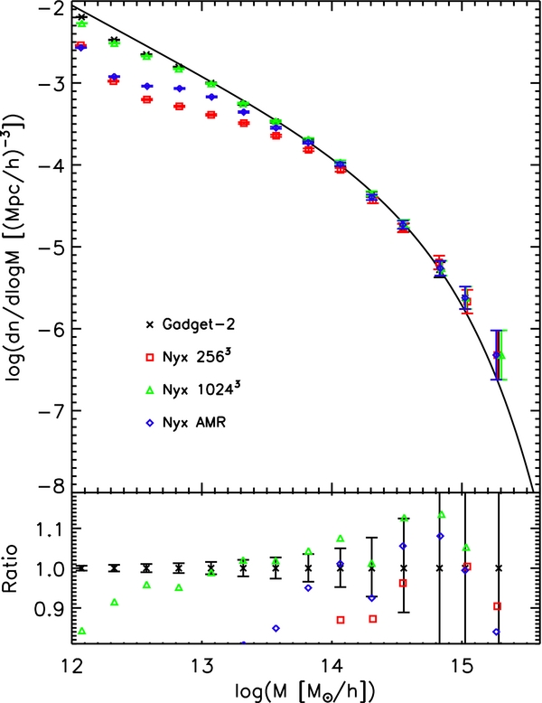
Figure 3. Halo mass function also shows good convergence with the increasing force resolution toward Gadget-2 results, run at higher resolution. The solid line is (Sheth & Tormen 1999) fit, shown here purely to guide the eye; ratios are taken with respect to Gadget as in the other plots.
Download figure:
Standard image High-resolution imageIn Figure 4 we present the correlation function for halos. Rather than looking at all halos together, we separate them into three mass bins. For the smallest halos we see the offset in the low resolution run, but even that converges quickly, in spite of the fact that the 10243 run still has fewer small-mass halos than the Gadget run done with force resolution several times smaller (Figure 3). Finally, in Figure 5 we examine the inner structure of halos. We observe excellent agreement between the AMR run and the uniform 10243 run, confirming the expectation that the structure of resolved halos in the AMR simulation match those in the fixed-grid runs. Overall, the agreement between the Nyx and Gadget-2 results is as expected, and is on a par with other AMR cosmology codes at this resolution as demonstrated in the Heitmann et al. papers.

Figure 4. Two-point correlation function of dark matter halos, separated in three mass groups. We see good agreement between the two codes, as well as rapid convergence even for halos sampled with a few tens of particles. We emphasize that halos in the range of 10–100 particles would not have been given serious consideration in a real application, but we show them here solely to examine differences between codes.
Download figure:
Standard image High-resolution image
Figure 5. Density profiles for the three most massive objects in the Gadget-2 run. The lines are the best fit NFW profile to the Gadget-2 run. We can see that the profiles from the AMR simulation closely match those of the uniform 10243 simulation.
Download figure:
Standard image High-resolution image6.2. Santa Barbara Cluster Simulations
The Santa Barbara cluster has become a standard code comparison test problem for cluster formation in a realistic cosmological setting. To make meaningful comparisons, all codes start from the same set of initial conditions and evolve both the gas and dark matter to redshift z = 0 assuming an ideal gas EOS with no heating or cooling ("adiabatic hydro"). Initial conditions are constrained such that a cluster (3σ rare) forms in the central part of the box. The simulation domain is 64 Mpc on a side, with the SCDM cosmology: Ω = Ωm = 1, Ωb = 0.1, h = 0.5, σ8 = 0.9, and ns = 1. A 3D snapshot of the dark matter density and gas temperature at z = 0 is shown in Figure 6. For the Nyx simulation we use the exact initial conditions from Heitmann et al. (2005), and begin the simulation at z = 63 with 2563 particles. Detailed results from a code comparison study of the Santa Barbara test problem were published in Frenk et al. (1999); we present here not all, but the most significant diagnostics from that paper for comparison of Nyx with other available codes. We refer the interested reader to that paper for full details of the simulation results for the different codes.

Figure 6. Santa Barbara cluster simulation. We show three orthogonal cuts through the box center showing dark matter density in blue-white colors. Superposed in red are iso-temperature surfaces of 107 K gas showing rich structure of intergalactic gas throughout the simulations domain.
Download figure:
Standard image High-resolution imageWe first examine the global cluster properties, calculated inside r200 with respect to the critical density at redshift z = 0. We find the total mass of the cluster to be 1.15 × 10¹⁵ M☉; Frenk et al. (1999) report the mean and 1σ deviation as (1.1 ± 0.05) × 1015 M☉ for all codes. The radius of the cluster from the Nyx run is 2.7 Mpc; Frenk et al. (1999) report 2.7 ± 0.04. The NFW concentration is 7.1; the original paper gives 7.5 as a rough guideline to what the concentration should be.
In Figure 7 we show comparisons of the radial profiles of several quantities: dark matter density, gas density, pressure, and entropy. Since the original data from the comparison project is not publicly available, we compare only with the average values, as well as the Enzo and ART data as estimated from the figures in Kravtsov et al. (2002). We also note that we did not have exactly the same initial conditions as in Frenk et al. (1999) or Kravtsov et al. (2002) and our starting redshift differs from that of Enzo (z = 30), so we do not expect exact agreement.

Figure 7. Left: density of dark matter (upper panel) and gas (lower panel); right: pressure (upper) and entropy (lower) profiles for the Santa Barbara cluster. Besides Nyx, we show the average from the original Frenk et al. 1999 paper, and results from two AMR codes, Enzo and ART.
Download figure:
Standard image High-resolution image
In the original code comparison, the definition of the cluster center was left to the discretion of each simulator, and here we adopt the gravitational potential minimum to define the cluster center. As in Frenk et al. (1999), we radially bin quantities in 15 spherical shells, evenly spaced in log radius, and covering three orders of magnitude—from 10 kpc to 10 Mpc. The pressure reported is p = ρgasT, and entropy is defined as s = ln (T/ρ2/3gas). We find good agreement between Nyx and the other AMR codes, including the well-known entropy flattening in the central part of the cluster. In sharp contrast to grid methods, smoothed particle hydrodynamics (SPH) codes find central entropy to continue rising toward smaller radii. Mitchell et al. (2009) made a detailed investigation of this issue, and have found that the difference between the two is independent of mesh sizes in grid codes, or particle number in SPH. Instead, the difference is fundamental in nature, and is shown to originate as a consequence of the suppression of eddies and fluid instabilities in SPH. (See also Abel 2011 for an SPH formulation that improves mixing at a cost of violating exact momentum conservation.) Overall, we find excellent agreement of Nyx with existing AMR codes.
7. CONCLUSIONS AND FUTURE WORK
We have presented a new N-body and gas dynamics code, Nyx, for large-scale cosmological simulations. Nyx is designed to efficiently utilize tens of thousands of processors; timings of the code up to almost 50,000 processors show excellent weak scaling behavior. Validation of Nyx in pure dark matter runs and dark matter with adiabatic hydrodynamics has been presented. Future papers will give greater detail on the implementation in Nyx of source terms, and will present results from simulations incorporating different heating and cooling mechanisms of the gas, as needed for increased fidelity in different applications. Scientific studies already underway with Nyx include studies of the Lyα forest and galaxy clusters. In addition, we plan to extend Nyx to allow for simulation of alternative cosmological models to ΛCDM, most interestingly dynamical dark energy and modifications of Einstein's gravity. The existing grid structure and multigrid Poisson solver should make it straightforward to extend the current capability to iterative methods for solving the nonlinear elliptic equations arising in those models.
This work was supported by Laboratory Directed Research and Development funding (PI: Peter Nugent) from Berkeley Lab, provided by the Director, Office of Science, of the U.S. Department of Energy under Contract No. DE-AC02-05CH11231. Additional support for improvements to BoxLib to support the Nyx code and others was provided through the SciDAC FASTMath Institute, funded by the Scientific Discovery through Advanced Computing (SciDAC) program funded by U.S. Department of Energy Office of Advanced Scientific Computing Research (and Office of Basic Energy Sciences/Biological and Environmental Research/High Energy Physics/Fusion Energy Sciences/Nuclear Physics). Calculations presented in this paper used resources of the National Energy Research Scientific Computing Center (NERSC), which is supported by the Office of Science of the U.S. Department of Energy under Contract No. DE-AC02-05CH11231.
We thank Peter Nugent and Martin White for many useful discussions.
Footnotes
- 4
We note that for small to moderate numbers of cores, pure-MPI runs can be significantly faster than runs using hybrid MPI and OpenMP. However, for the purposes of this scaling study we report only hybrid results.