


ABSTRACT
The ribbon observed by the Interstellar Boundary Explorer (IBEX) mission is a narrow, ∼20° wide feature that stretches across much of the sky in the global flux of energetic neutral atoms from the outer heliosphere. The ribbon remains an enigma despite its persistence after 3 years of IBEX observations and after almost a dozen theories that attempt to explain it. While each theory that has been posed has its strengths, each one also contradicts IBEX observations or demonstrates significant flaws in internal consistency. Here, we present a new theory that is different than any of the existing ideas and yet accounts for many of the key observations. We argue that the ribbon could be produced by a spatial region in the local interstellar medium where newly ionized atoms are temporarily contained through increased rates of scattering by locally generated waves in the electromagnetic fields. The particles in the ribbon are created predominantly from neutralized solar wind and neutralized pickup ions from inside the solar wind termination shock.
Export citation and abstract BibTeX RIS
1. INTRODUCTION
The Interstellar Boundary Explorer (IBEX) mission was launched on 2008 October 19, with the central objective of discovering the global interaction between the solar wind and the local interstellar medium (McComas et al. 2009b). The first global maps of the heliosphere in ENAs were presented in four papers (McComas et al. 2009a; Funsten et al. 2009b; Fuselier et al. 2009; Schwadron et al. 2009a), and the first measurements of low-energy interstellar oxygen, helium, and hydrogen atoms were also provided (Möbius et al. 2009). In the same issue, Krimigis et al. (2009) showed higher energy results from INCA. The IBEX sky maps showed striking differences between observations and predictions from models (Schwadron et al. 2009a).
The IBEX maps showed the presence of a narrow ribbon (∼20° wide) of elevated ENA emissions (McComas et al. 2009a; Funsten et al. 2009b; Fuselier et al. 2009) that forms a circular arc centered on ecliptic coordinate (long., lat.) ∼(221°, 39°), likely near the local interstellar (LISM) magnetic field direction (Schwadron et al. 2009a). Based on comparisons with models of the compressed plasma in the outer heliosheath, the ribbon appears to line up well with directions in the sky where the radial line of sight (r) is roughly perpendicular to the compressed LISM magnetic field (B) so that B · r ≈ 0 (McComas et al. 2009a; Schwadron et al. 2009a). One of the surprising features of the ribbon is that the spatial distribution appeared to be relatively independent of energy after subtracting the distributed emissions (globally distributed flux) outside the ribbon (Fuselier et al. 2009). The energy spectral slope of the observed fluxes appeared to be ordered predominantly by ecliptic latitude (McComas et al. 2009a; Funsten et al. 2009b).
The ribbon is a distinct feature. It has properties such as a narrow angular width and an energy distribution that are distinct from the globally distributed flux. In this paper, we explore a new physical mechanism to explain the key observational features of the ribbon.
The ribbon's overall stability and the existence of some time variability (McComas et al. 2010) provide important information on the true source of this feature. There is also time variation observed in the surrounding globally distributed flux. In fact, one of the most striking features is a reduction in the overall flux across the maps at all energies (McComas et al. 2010). McComas et al. (2012) showed that after 3 years, both the globally distributed flux and the flux in the ENA ribbon has continued to decrease. This reduction in flux appears qualitatively consistent with a known reduction in the solar wind flux in the recent solar minimum (McComas et al. 2008; Schwadron & McComas 2008).
We briefly review the mechanisms proposed to explain the ribbon (earlier reviews of these mechanisms were provided by McComas et al. 2010 and Schwadron et al. 2011, and the first six of these mechanisms were originally suggested by McComas et al. 2009a).
- 1.McComas et al. (2009a) and Funsten et al. (2009b) found that the slopes in the first IBEX maps were ordered by latitude. It follows that the same plasma population and, by extension, similar processes generate both the ribbon and the globally distributed flux. The ribbon is found in regions where the j × B force is maximized in the outer heliosheath (Schwadron et al. 2009a), leading to the idea that the ribbon may somehow arise from compression of material in that region, a cavity on the heliopause, or through extrusions associated with enhanced tension and magnetic pressure that might also explain the fine structure observed in the ribbon (McComas et al. 2009a).
- 2.The enhanced j × B force in the outer heliosheath leads to compression of the LISM magnetic field. If the first-adiabatic invariant is conserved, then compression causes pitch angles aligned more closely perpendicular to the magnetic field, leading naturally to enhanced emissions along the region where B · r ∼ 0. If these compressions are generated in the outer heliosheath, then we expect to see a different energy spectrum in the ribbon as compared to the distributed flux. The energy spectrum should reflect the source population. In this case, the angular distribution in the ribbon would be approximately independent of energy (Schwadron et al. 2009a).
- 3.The charge-exchange process also creates a neutral solar wind. The neutralized solar wind from inside the termination shock moves predominantly outward in the radial direction. When these neutral atoms travel beyond the heliopause there is some probability that they will become ionized through charge-exchange. When this happens, a newly born ion begins to gyrate about the local magnetic field. Around regions where B · r ∼ 0, newly created pickup ions rotate through a special gyrophase where the ion is moving directly inward toward the Sun and toward IBEX. If another charge-exchange collision occurs when the ion has this special inward-directed gyrophase, then an ENA is created that can be observed by IBEX. This mechanism was suggested by McComas et al. (2009a) and has subsequently been included in a number of models (Heerikhuisen et al. 2010; Chalov et al. 2010). The mechanism produces ENAs from the outer heliosheath and even beyond the heliosphere in the LISM. The resulting energy distribution is peaked at around the solar wind energy, >1 keV in the supersonic solar wind.
- 4.Magnetic reconnection along the heliopause induced by enhanced forces would create locations where hot plasma from the inner heliosheath can leak out into the outer heliosheath. The reconnection itself may also lead to substantial heating. Suess (2004) showed that the opposite orientation of magnetic field from the inner heliosheath and magnetic field in the local interstellar medium occurs on thin bands (several AU) that essentially paint the heliopause. Therefore, enhanced j × B forces may naturally cause magnetic reconnection along the heliopause within the bands where magnetic field lines oppose one another. This form of reconnection, if it causes the ribbon, may lead to a harder energy spectrum through heating associated with magnetic reconnection. However, it might also lead to similarities in the energy spectrum in the ribbon as compared to the distributed flux since material from the inner heliosheath would leak out into the outer heliosheath and cause enhanced ENA emission through a lengthened line of sight (LOS).
- 5.It is also possible that the ribbon results, at least in part, from accelerated pickup ions near the termination shock. This concept would lead to a peak in the ribbon of around 1–16 keV due to pickup ions (∼4–16 keV) and reflected solar wind ions (1–4 keV).
- 6.Raleigh–Taylor and/or Kelvin–Helmholtz instabilities on the heliopause may operate preferentially where j × B forces are large, thereby explaining the ribbon. We expect fine structure associated with these processes because they are turbulent in nature. In this mechanism, it is difficult to predict how the ENA energy spectrum would differ from other emission regions in the inner heliosheath. We might expect some similarity to predictions from magnetic reconnection: enhanced ENA emission arises from both additional heating in these regions and lengthened LOS. Therefore the energy spectrum would likely be harder than other emission regions from the inner heliosheath, particularly near the nose where the dynamic pressure is largest.
- 7.A hypothesis beyond the concepts introduced by McComas et al. (2009a) is that the ribbon may arise from the interaction of the Local Interstellar Cloud (LIC) with the Local Bubble (Grzedzielski et al. 2010). Because the Local Bubble has a temperature of ∼106 K, we might expect a peak or roll-over in the energy spectrum near ∼0.15 keV, were it not for the strong extinction in the intervening LIC layer, which only allows ions of higher energies to be observed by IBEX. In fact, it is mostly the ENAs originating from a suprathermal ion component in the Local Bubble that will form the ribbon in this mechanism. Hence this mechanism requires a ∼1% suprathermal component in the Local Bubble plasma.
- 8.Another concept for the ribbon is that it is generated by pickup ions accelerated at the termination shock: the anomalous cosmic ray (ACR) induced component (Fahr et al. 2011). Shock-generated ACRs can diffuse inward from the shock and then get modulated in energy due to adiabatic cooling processes. The loss of particle energy and associated decrease of the spatial diffusion coefficient leads to loss of particle diffusive mobility while the particles propagate inward. Subsequently, these particles are co-convected with the bulk solar wind to increasing solar distances. The fluxes predicted by this mechanism likely contribute to the ENAs observed by IBEX, but cannot account for the dominant features in the IBEX ribbon.
- 9.Siewert et al. (2012) further studied the concept of shock accelerated particles using kinetic and multifluid theories describing the solar wind termination shock (TS) transition. This allowed derivation of the downstream pickup ion (PUI) distribution function as a function of shock properties, such as the local magnetic field tilt angle and the compression ratio. The kinetic model provided a formulation of latitude- and longitude-dependent spectral intensities between 1 and 100 keV. After converting shock-processed PUIs to ENAs by charge exchange with cold H-atoms, the predicted keV ENA fluxes are of the same order of magnitude as those observed by IBEX and a narrow feature of enhanced emission that could, in principle, be related to the IBEX ribbon.
All the models for the ribbon are ultimately tested by their ability to reproduce the IBEX observations. Key observations include the following.
- 1.The ribbon itself is a fairly narrow feature at low energies. For example, at ∼1 keV the ribbon has an FWHM of ∼20°. This width is variable from ∼10°–40° depending on the position along the ribbon (Schwadron et al. 2011).
- 2.The ribbon width broadens with increasing energy. For example, at ∼4.29 keV the FWHM of the ribbon increases to 40°–70° (Schwadron et al. 2011).
- 3.There may be ordering of the ribbon by B · r = 0. This relationship was detailed by (Schwadron et al. 2009a) on the basis of comparison between a modeled heliosphere and IBEX observations. The comparison suggests a direct relationship between the ribbon and the local interstellar magnetic field; however, the direction and strength of the interstellar magnetic field remain unknown.
- 4.The energy distribution of the ribbon was studied and found to have a pronounced knee in comparison to the globally distributed flux (Schwadron et al. 2011). The knee in the ribbon varies with latitude such that a lower energy knee (∼1 keV) exists at low latitudes and a higher energy knee (∼4 keV) at higher latitudes (Schwadron et al. 2011; McComas et al. 2012). This observation (as exemplified in Figure 1 from McComas et al. 2012) strongly supports a solar wind related source for the ribbon since the energies are consistent with a slower wind (∼450 km s−1) at low latitudes and a faster wind (∼750 km s−1) at high latitudes, which is a known ordering of solar wind near solar minimum conditions (McComas et al. 2000).
- 5.The existence of fine structure within the ribbon (McComas et al. 2009a), which suggests that the physical properties of the ribbon exhibit small-scale spatial structure and possibly rapid small-scale variations.
Thus far, the neutral solar wind (mechanism 3 above) is the only source mechanism suggested that has intrinsic ordering by B · r = 0 and should reflect the latitudinal ordering of the solar wind. Heerikhuisen et al.'s (2010) model requires stability of the pickup ring over years for it to contribute a sufficiently large source to explain the ribbon. However, Florinski et al. (2010) showed that the pickup ring needed to create the ribbon is inherently unstable. Gamayunov et al. (2010) suggest ways in which the spectrum of electromagnetic waves may allow metastability of the pickup ring. Nevertheless, stability of the ring-distribution needed for the ribbon in the neutral wind scenario remains a challenge to this source mechanism.
In this paper, we present an extension of the neutral solar wind conjecture, which does not require long-term stability of the pickup ring. We develop a physical model of the ribbon that is quite simple and shows consistent signatures that agree quantitatively with observations.
2. ION RETENTION THROUGH RAPID SCATTERING
The ion retention mechanism starts with the creation of ions within the local interstellar medium from neutral solar wind as described by McComas et al. (2009a), Heerikhuisen et al. (2010), and Chalov et al. (2010). Newly born ions begin to gyrate about the local interstellar magnetic field, forming a so-called ring distribution (see Figures 1 and 2). The ring distribution has a specific ion velocity component parallel (v∥) and perpendicular (v⊥) to the magnetic field: v∥ = vμ and  where μ is the cosine of the ion pitch angle relative to the magnetic field. The fate of the pickup ion depends sensitively on the initial parallel component of the ion velocity (shown in Figure 2). We make use of the wave-particle instability of the pickup ring (e.g., Lee & Ip 1987; Sagdeev et al. 1987; Karimabadi et al. 1994). There are two important regimes for the initial parallel velocity to consider.
- 1.In the first regime, the magnitude of the parallel speed is smaller than the Alfvén speed |v∥| < vA (see the middle panel of Figure 2). In this case, ions interact with parallel propagating Alfvén waves moving in either direction along the field and through the scattering by these waves decrease their pitch angle. If ions with positive parallel velocities are scattered by waves with negative Alfvén speeds (or vice versa), then the ions can lose energy in the plasma reference frame and thereby enhance the intensity of the waves. This is the classic case of plasma-wave instability that rapidly creates a bispherical distribution for the ions. This process inherently destroys the streaming of pickup ions and causes relatively short scattering mean free paths for the ions, which inhibits diffusion.
- 2.In the second regime, the initial magnitude of the parallel velocity exceeds Alfvén speed. In this case, either v∥ > vA (top panel) or v∥ < −vA (bottom panel). We describe the situation for v∥ > vA, and note that the opposite case is identical with a change of sign for the velocity components. In the scattering process, the typical resonance condition applies: for waves with positive Alfvén speed, k(v∥ − vA) = Ω and for waves with negative Alfvén speed, k(v∥ + vA) = Ω, where Ω is the particle gyrofrequency. For the waves with negative Alfvén speed, the initial pickup ring resonates with wavenumber ki − = Ω/(vi + vA) where vi is the initial parallel velocity. For, k− > ki −, waves become unstable since pickup ions scatter to smaller pitch angles with larger parallel velocities, thereby losing energy in the plasma frame. For the waves with positive Alfvén speed, the resonance with the initial pickup ring is at wavenumber ki + = Ω/(vi − vA) and for k+ < ki +, pickup ions scatter to larger pitch angles (with smaller parallel velocities), thereby losing energy in the plasma frame and causing wave intensities at increasing wavenumbers to grow. However, there is a limit for this scattering process: as the parallel velocity approaches the Alfvén speed, v∥ → vA, the resonant wavenumbers must grow, k+ → ∞, and the wave power, typically an inverse power law with wavenumber, drops precipitously. The result is that the waves that are unstable cause scattering only for v∥ > vA and the ion distributions become approximately uniform in only one hemisphere. This situation leads to a large streaming of such ions at a speed of ∼v/2, where v is the initial speed of the ions at pickup. The hemispheric distribution is rapidly achieved through the scattering process and the resultant ratio of parallel to perpendicular temperature, T⊥/T∥ ∼ 1, is well below the stability limit for the production of ion cyclotron waves (ion-cyclotron instabilities arise for T⊥/T∥ > 2, e.g., Gamayunov et al. 2010).

Figure 1. (From McComas et al. 2012) Schematic diagram of (left) the distribution of solar wind speed organized by heliolatitude in a solar minimum configuration (McComas et al. 2000) and (right) the ENA generation from neutral solar wind in regions where the compressed interstellar magnetic field is roughly perpendicular to the almost radial outflowing neutral atoms from the solar wind. The three Mollweide projections (right) show full-sky projections of observed differential ENA flux (in units of (cm2 s sr keV)−1) by IBEX.
Download figure:
Standard image High-resolution image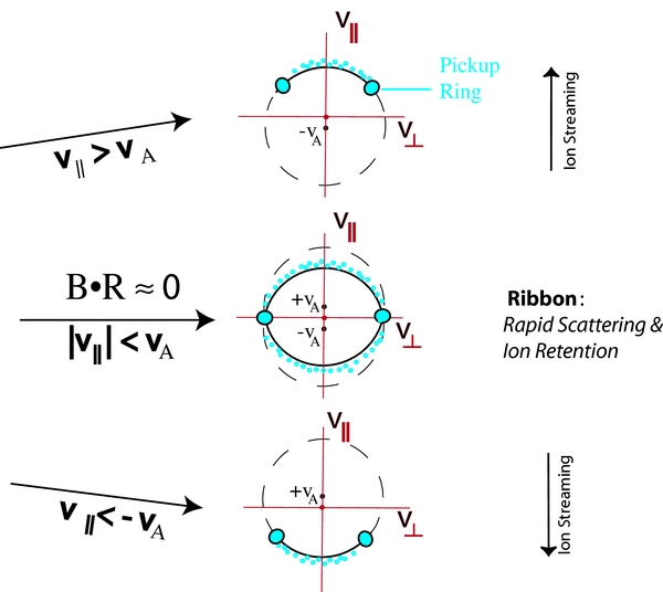
Figure 2. Fundamental regimes of ion pickup, scattering and Alfvén wave instability. When atoms first become ionized, they begin to gyrate about the local magnetic field in a pickup ring with a specific pitch angle and a velocity component parallel to the local magnetic field. The top and bottom panels show the situation in which the magnitude of the initial parallel velocity component exceeds the Alfvén speed. In the top panel, ion scattering to smaller pitch angles causes an increase in streaming and amplifies the Alfvén waves with negative Alfvén speed. To the contrary, scattering by these inward Alfvén waves to increased pitch angles damps these waves. While there can be some amplification of waves in the range vi > v∥ > vA (where vi is the initial parallel velocity component), the resonance condition implies that the scattering occurs via waves of increasing wavenumber and decreasing wave power. As v∥ → vA, the probability of wave scattering becomes extremely small. As a result, the scattering leads to the approximately hemispheric pitch-angle distribution shown in the top panel. In the middle panel, we show the situation in which the initial pickup ring exists for −vA ⩽ vi ⩽ vA. In this case, scattering to increased parallel velocities leads to enhancement of Alfvén waves with negative Alfvén speeds, and scattering to decreased parallel velocities leads to enhancement of Alfvén waves with positive Alfvén velocities. This is the classic case of an unstable pickup ion ring that rapidly scatters forming a nearly isotropic ion distribution, as shown. The bottom panel mirrors the top panel. In this case, the initial pickup ring has parallel velocities v∥ < −vA. Scattering by Alfvén waves with positive Alfvén speeds rapidly forms a hemispheric distribution with negative parallel velocities. In the top and bottom panels, ions stream predominantly away from the ribbon, and Alfvén waves travel into the strong scattering region, causing even more rapid scattering.
Download figure:
Standard image High-resolution imageConsiderable observational evidence for hemispheric distributions has resulted from direct studies of pickup ion distributions in the solar wind with the Ulysses/SWICS instrument (Gloeckler et al. 1992) and the SOHO/CELIAS instrument (Hovestadt et al. 1995). Data from the CELIAS instruments were used in the measurement of the velocity distribution of singly charged helium ions. These observations were favorably compared to the predictions of a hemispheric model of pitch-angle diffusion (Saul et al. 2007). In Fisk et al. (1997), SWICS was used to study correlated statistical fluctuations in pickup protons and singly charged pickup helium. The observations indicated that the pickup distributions were roughly uniform in the outward facing hemisphere (away from the Sun along the interplanetary magnetic field). The apparent implication is that the rate of pickup ion scattering near 90° pitch angle is greatly diminished. In both of these sets of observations by Ulysses/SWICS and SOHO/CELIAS, the difficulty of scattering through 90° pitch angle led to large scattering mean free paths and hemispheric pitch-angle distributions. Numerous subsequent models (e.g., Isenberg 1997; Schwadron 1998; Lu & Zank 2001) have made use of the hemispheric pitch-angle distribution to understand transport of pickup ions in the heliosphere.
The considerations of Alfvén wave instabilities and wave-particle interactions result in a picture (Figure 3) where ions are rapidly scattered and therefore diffusively inhibited only in a region centered on the line where B · r = 0. This region of Alfvén retention has a width defined by the condition that |v∥| < vA. If we take a density of LISM of 0.07 cm−3 (Frisch et al. 2009), an LISM magnetic field strength of 3 μG (Schwadron et al. 2011), and a compression factor of 2.5, then the Alfvén speed is vA ∼ 40 km s−1 in the compressed LISM just beyond the heliopause. At ∼1 keV, ion speeds are v ∼ 440 km s−1 and the pitch angle where the v∥ ∼ vA is θ ∼ acos(vA/v) ∼ 85°. This yields an "Alfvén spread" of ΔαA ∼ 10° (the region of instability for positive Alfvén speeds extends for pitch angles from 85° to 90° and the region of instability for negative Alfvén speeds extends for pitch angles from 90° to 95°) over which waves move bi-directionally. For fast wind with speed ∼750 km s−1, the Alfvén spread is smaller, ΔαA ∼ 6°.

Figure 3. Basic picture of Alfvén retention. Neutral atoms from the solar wind and pickup ions (PUIs) travel out beyond the heliopause where they become ionized and begin to gyrate about the local interstellar magnetic field. If the pitch angles of these newly picked up ions have speeds parallel to the magnetic field that are smaller than the Alfvén speed, then Alfvén waves are unstable and are amplified through scattering of the initial pickup ring. As a result, for ions with initial parallel speeds less than the Alfvén speed, there is rapid scattering of these ions, which leads to their retention near the region B · r = 0. Conversely, for ions with parallel speeds greater than the Alfvén speed, the ion distributions tend to scatter only within the heliosphere in which they are picked up. This leads to ion streaming in the direction away from the B · r = 0 position and the amplification of Alfvén waves that move toward B · r = 0 position. The retention of ions near the B · r = 0 positions could be the key missing element in the creation of the IBEX ribbon.
Download figure:
Standard image High-resolution imageThe fact that the ion retention region from solar wind neutrals narrows with increasing energy appears to contradict observations of the ribbon. We will show however that the broadening of the ion retention region at increased energies follows naturally from a quantitative model of ion retention (Section 3). The increased mobility of higher energy particles leads to enhanced diffusion within the retention region, which thereby broadens the region of increased density.
The Alfvén spread ΔαA ∼ 10° is calculated from a neutral beam-like solar wind source ionized on an ideal planar magnetic field. The fact that the solar wind has a finite temperature (several eV in the outer heliosphere) leads to some dispersion of the neutral solar wind over an angle range of ΔαV ∼ 4° (Gamayunov et al. 2010), which we refer to as a "velocity spread." Combining the velocity and Alfvén spread, we find a minimum intrinsic width of the ion retention region of ∼10°–14° for ions near 1 keV.
In addition to the specific considerations regarding the source of ions, there are several additional factors that broaden the retention region (e.g., Heerikhuisen & Pogorelov 2011). The interstellar magnetic field is deflected as it wraps around the heliopause. This deforms the region where B · r = 0 from a great circle to a locus shifted by ∼10° inside the great circle (McComas et al. 2009a; Schwadron et al. 2009a). Since the ribbon is integrated along the LOS, we expect to see some shift of the in the structure, which broadens the ribbon and potentially produces fine structure (McComas et al. 2009a) due to the superposition of shifted retention regions.
3. ION RETENTION MODEL
In this section, we address the expected ENA fluxes and densities from the supersonic solar wind that provide sources for the retention region. In the Appendix, we solve for the differential flux of ENAs from neutralized supersonic solar wind. There are two fundamental regimes solved for: within the ion retention region rapid scattering confines ions and outside the ion retention the scattering becomes weak and the scattering mean free path becomes large. Therefore, the ion retention region accumulates larger suprathermal ion densities and the distribution function becomes roughly isotropic. Outside the ion retention region, the density falls off and the distribution becomes highly anisotropic with a strong field-aligned streaming away from the retention region.
The parameters controlling the differential flux of ENAs can be detailed based on the major processes behind the creation of ENAs from the retention region.
- 1.The process starts with the neutral solar wind which has a flux that depends on three factors: the flux of solar wind protons at 1 AU, F1 ∼ 3 × 108 cm−2 s−1 (McComas et al. 2000), the neutral density of hydrogen atoms in the heliosphere nH ∼ 0.12 cm−3 (Gloeckler 1996) that charge-exchange with solar wind, and distance from the Sun (the flux falls off approximately as 1/R2 beyond the termination shock).
- 2.Neutral solar wind becomes ionized in the outer heliosheath due to charge-exchange with protons that we take to have density np-OHS = 0.18 cm−3 based on an LISM proton density of 0.07 cm−3 and a compression factor of 2.5 in the outer heliosheath (Schwadron et al. 2009a).
- 3.Once ionized, newly created protons travel along magnetic field lines, but their lifetime τx = 1/(σnH-OHSv) is again limited by charge-exchange. Here, nH-OHS ∼ 0.22 cm−3 is the H density in the outer heliosheath. Once converted back to ENAs, those atoms traveling inward toward IBEX may be detected. The net differential flux observed also depends on the LOS length that we take to be 100 AU.
Parameters used here for the densities of within the heliosheath are motivated by model results in Müller et al. (2008).
The scattering length λ can be related to the pitch-angle diffusion coefficient found from quasi-linear theory (e.g., Schlickeiser 1989; Gamayunov et al. 2010) based on a prescribed Kolmogorov magnetic power spectrum B2(k) ∼ 2B2slabkmin2/3/[5(k5/3min + k5/3)] where k is the wavenumber, the parameter lb = 1/kmin is the break wavelength separating the energy range in the energy containing wave power spectrum from the inertial range, and Bslab is the field magnitude of slab fluctuations in the wave field. The formula given by Schlickeiser (1989) assumes equal power for the forward and backward propagating waves. The scattering mean free path is largely controlled by the low values of the scattering operator Dμμ in the limit that |μ| → 0, where μ is the pitch-angle cosine. In this, limit we find that

where Ω = qB/(mc) is the ion gyrofrequency. The major uncertainties here are the relative magnitude of the slab fluctuations (Bslab/B) and the break wavelength lb. Gamayunov et al. (2010) argue that the background interstellar turbulence should have relatively large values for lb (100's of AU) while small-scale self-generated waves should have extremely small values lb > vA/Ω. Using Equation (1), we estimate the scattering mean free path by λ ∼ v/Dμμ(|μ| ∼ 0). While definitive parameters for lb and (Bslab/B) are not currently available at this distance, it is useful to work out a representative case. For example, with lb ∼ 0.005 AU and (Bslab/B) ∼ 0.1 the scattering mean free path is ∼1 AU. This value for the scattering mean free path does not appear unreasonable given typically observed mean free paths of ∼1–2 AU at keV energies (e.g., Gloeckler et al. 1995) in the inner heliosphere at ∼4 AU where field strengths of ∼5–10 μG are typical and comparable to the field strengths in the outer heliosheath.
Our model for the ribbon assumes that the neutral solar wind has a Gaussian speed distribution, ![$f_{{\rm SW}-v} \propto \exp [ -(v-u_\mathrm{SW})^2/ \Delta u_\mathrm{SW}^2 ]/(\sqrt{\pi }\Delta u_\mathrm{SW}))$](https://content.cld.iop.org/journals/0004-637X/764/1/92/revision1/apj456852ieqn2.gif) where ΔuSW = 250 km s−1 and uSW is the mean neutral wind speed that varies with ecliptic latitude. Sokół et al. (2012) have developed detailed empirical fits to the latitude solar wind distribution in each year from 1990 through 2011 using Ulysses, the OMNI 2 database, and remote sensing observations of interplanetary scintillations. In using these fits in our model, we must take into account a ∼4 year transit time delay between observations of solar wind in the inner heliosphere and the IBEX observations of the ribbon. The transit time delay arises from the ∼1.5 year propagation time of a 1 keV neutral H atom from the inner heliosphere out to 150 AU, the ∼1–2 year retention time of ions from solar wind that occupy the retention region and eventually undergo charge-exchange, and the ∼1.5 year propagation time of an ENA back to IBEX. At 4 keV, this delay time is shorter, ∼2–3 years. Accounting for a ∼ 4 year transit delay, we use solar wind observations in 2005 to model the first IBEX maps observed in 2009. We also account for mass-loading of solar wind by subtracting 150 km s−1 from the 2005 solar wind speeds.
where ΔuSW = 250 km s−1 and uSW is the mean neutral wind speed that varies with ecliptic latitude. Sokół et al. (2012) have developed detailed empirical fits to the latitude solar wind distribution in each year from 1990 through 2011 using Ulysses, the OMNI 2 database, and remote sensing observations of interplanetary scintillations. In using these fits in our model, we must take into account a ∼4 year transit time delay between observations of solar wind in the inner heliosphere and the IBEX observations of the ribbon. The transit time delay arises from the ∼1.5 year propagation time of a 1 keV neutral H atom from the inner heliosphere out to 150 AU, the ∼1–2 year retention time of ions from solar wind that occupy the retention region and eventually undergo charge-exchange, and the ∼1.5 year propagation time of an ENA back to IBEX. At 4 keV, this delay time is shorter, ∼2–3 years. Accounting for a ∼ 4 year transit delay, we use solar wind observations in 2005 to model the first IBEX maps observed in 2009. We also account for mass-loading of solar wind by subtracting 150 km s−1 from the 2005 solar wind speeds.
The ENA flux and ion retention densities depend on the distance of the source. For simplicity, we take a heliopause with an elliptical shape, with a nose at 150 AU, flanks at 225 AU, and a tail at 450 AU (Müller et al. 2008). We assume the TS is 2/3 the distance to the heliopause, which places the TS nose at 100 AU, the TS flanks at 150 AU, and TS tail at 300 AU.
Modeled densities (Figures 4 and 5) demonstrate the large suprathermal population contained near the ion retention region. The density corresponds to that from the "reverse" hemisphere comprised of pitch angles with parallel velocity components directed toward the center of the retention region along the magnetic field. This reverse hemisphere covers a range of directions including those directed back toward IBEX. Therefore, protons within this reverse hemisphere can charge-exchange to become ENAs detected by IBEX. Modeled densities also reveal a broadened region of enhancement at higher energies (e.g., 2–6 keV). This broadening is due to the increased mobility of ions at higher energies that allows the density to spread out more effectively through the retention region.
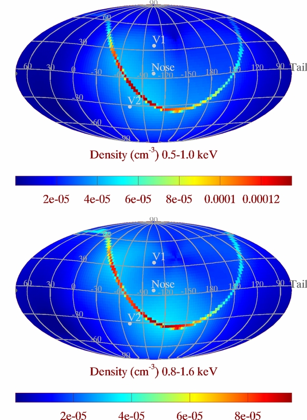
Figure 4. Sky maps of density near the heliopause integrated over the indicated energy ranges near IBEX-Hi energy steps 2 and 3 for the top and bottom panels, respectively. While these densities are lower than typical ISM densities, they represent large densities in the suprathermal energy range. Note that the density shown corresponds to that from the "reverse" hemisphere directed toward the center of the retention region along the magnetic field. This reverse hemisphere covers a range of directions including those directed back toward IBEX. Therefore, protons within this reverse hemisphere can charge-exchange to become ENAs detected by IBEX.
Download figure:
Standard image High-resolution image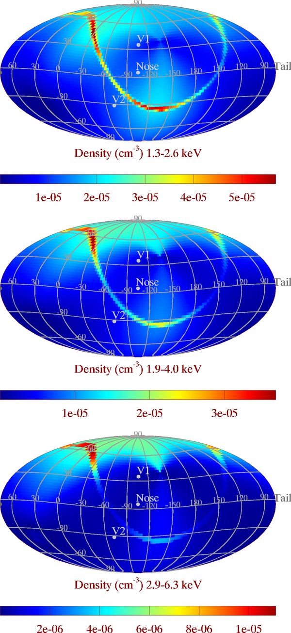
Figure 5. Sky maps of density near the heliopause integrated over the indicated energy ranges near IBEX-Hi energy steps 4, 5, and 6 (from top to bottom panels).
Download figure:
Standard image High-resolution imageThe panels in Figures 6 and 7 show the ENA flux over the top five energy passbands of IBEX-Hi. Left panels show modeled fluxes, whereas the right-hand panels show IBEX observations of the ribbon (Schwadron et al. 2011). We use the IBEX-Hi response function (Schwadron et al. 2009b; Funsten et al. 2009a) to integrate over acceptance angles and acceptance energies for each of the IBEX-Hi electrostatic analyzer (ESA) steps.

Figure 6. Ion retention model at energy steps 2 and 3 of the IBEX-Hi instrument. The ion retention model has been integrated over energy and angle with the IBEX-Hi response function from Schwadron et al. (2009b) and Funsten et al. (2009a). IBEX observations of the ribbon (Schwadron et al. 2011) are also shown (right panels) for comparison.
Download figure:
Standard image High-resolution image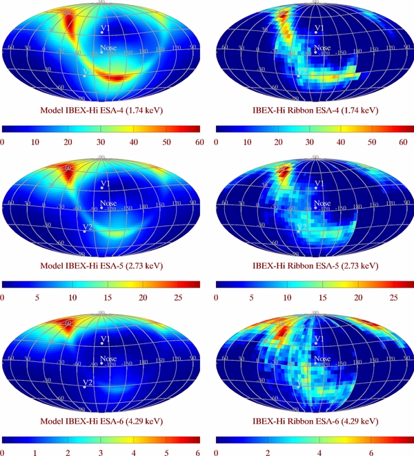
Figure 7. Ion retention model (left panels) at energy steps 3, 4, and 6 of the IBEX-Hi instrument. IBEX observations of the ribbon (Schwadron et al. 2011) are also shown (right panels) for comparison.
Download figure:
Standard image High-resolution image
4. SUMMARY AND CONCLUSIONS
We have developed a model for the IBEX ribbon based on spatial ion retention within the local interstellar medium. The fundamental basis of the model is the enhanced ion scattering that occurs when ions are picked up almost perpendicular to the interstellar magnetic field. In this case, ions have free energy that they release to magnetohydrodynamic waves as the ion distributions are pitch angle scattered by the waves. The wave creation then causes more rapid ion scattering. Thus, the initial ion distributions are unstable in the regions where ions are picked up roughly perpendicular to the magnetic field (Florinski et al. 2010).
In regions where ions are picked up with substantial initial velocities parallel to the magnetic field (|v∥| > vA), the pickup ion ring instability only amplifies waves moving in one direction (waves moving in the opposite direction from ions along the field are amplified), and the subsequently incomplete scattering of the pickup ring leads to ion distributions with substantial streaming of ions away from the retention region. The result is a narrow band, the ribbon, where efficient scattering of pickup ions retains ions spatially close to regions where the radial LOS is roughly perpendicular to the interstellar magnetic field, as observed (McComas et al. 2009a; Schwadron et al. 2009a).
The ion retention model with a source from solar wind neutrals has an intrinsic width of about 10° at 1 keV, which is narrower than the ∼20° observed width at this energy. However, some broadening occurs due to diffusion of particles both within and outside the retention region. Variations in the interstellar magnetic field will also likely broaden the ribbon. These variations are unlikely to cause larger deviations in the magnetic field since the plasma beta is close to unity (the Alfvén speed and the interstellar flow speed are of similar magnitude in the outer heliosheath).
We have only considered the supersonic solar wind source of neutrals, which is a collimated neutral beam. Other sources of neutrals such as pickup ions from inside the termination shock would not be so strongly collimated and therefore would contribute to a broadening of the ribbon in both angle and energy.
The diffusive process itself confines ions over a very limited spatial region, with peaks in flux that have a smaller angular extent than the IBEX field of view. This factor may lead to the observation of small-scale structure (McComas et al. 2009a). Further, since the charge-exchange lifetime is ∼1.7 year at 1 keV, we expect significant time variation of the ribbon even on the small 6 month timescales over which IBEX creates neutral atom maps.
The ion retention mechanism reduces the mobility of ions near the center of the IBEX ribbon. Therefore, ion retention is a spatial effect and is fundamentally different from previous mechanisms (e.g., McComas et al. 2009a; Heerikhuisen et al. 2010) that have identified the role of special pickup ion velocity distributions with ions preferentially near 90°. While the model detailed here is very specific concerning the mechanism of spatial confinement, there are likely additional effects that can spatially isolate ions near the ribbon and additional source populations that contribute to the excess of ions in this region. Ion retention is therefore intended to encompass the varied mechanisms that allow spatial confinement of ions near the IBEX ribbon.
Model results here show that the ENA signatures from the retention region have characteristic variations that reflect the solar wind source with a slower wind at low latitudes and a faster wind at high latitudes during solar minimum. In this context, it will be interesting to observe the evolution of the IBEX ribbon near solar maximum. Model results also show that the high latitude signatures of fast solar wind in the ribbon should transition to slow solar wind signatures near solar maximum. While these results are a natural prediction of the ion retention model, it is also likely that any ribbon mechanism based on a neutral solar wind source would have a similar organization as a function of heliolatitude.
Thus, this paper provides a critical missing physical component that explains many properties of the IBEX ribbon. The spatial retention of ions in the local interstellar medium due to rapid scattering of ions picked up roughly perpendicular to the magnetic field leads to a region of enhanced ENA flux where B · r ≈ 0.
We are deeply indebted to all of the outstanding people who have made the IBEX mission possible. This work was carried out as a part of the IBEX project, with support from NASA's Explorer Program.
APPENDIX: SUPERSONIC SOLAR WIND SOURCE OF THE RETENTION REGION
The supersonic solar wind model of ion retention is the simplest to develop because the source is beam-like. We start by writing down an expression for the production rate of protons within the retention region:
where F1 is the solar wind flux at r1 = 1 AU, R is the radial distance to the retention region, nH is the hydrogen density inside the termination shock, σ is the charge-exchange cross-section for hydrogen, and np-OHS is the total proton density near the retention region in the outer heliosheath. This expression is derived by recognizing first that the number of solar wind protons within a solid area element dΩ is approximately constant with radial distance. The fraction of these protons that becomes neutralized over the distance to the termination shock (at RTS) is (nHσRTS). The flux of neutralized solar wind into the retention region is then FN = F1(r21/R2)nHσRTS and the proton production rate is this neutral flux times σnp-OHS, which yields Equation (A1).
Assuming that the protons associated with the supersonic solar wind source are scattered into a nearly isotropic distribution, we can identify a source rate for the isotropic distribution function from A1:
Therefore, the isotropic distribution source function is
where δ(x) is the Dirac delta function. While this expression is correct for a fixed solar wind speed, the solar wind itself exhibits a range of speeds. In this context, it is appropriate to replace the delta function with a distribution of solar wind speeds, centered about a mean speed. We assume a Gaussian distribution about a mean speed uSW and a spread of speeds ΔuSW, so that ![$\delta (v-u) \rightarrow \exp \left[ -(v-u_\mathrm{SW})^2/ \Delta u_\mathrm{SW}^2 \right]/(\sqrt{\pi }\Delta u_\mathrm{SW})$](https://content.cld.iop.org/journals/0004-637X/764/1/92/revision1/apj456852ieqn3.gif) . This leads to the following expression for the isotropic source function within the retention region:
. This leads to the following expression for the isotropic source function within the retention region:
A model for ion fluxes within the ion retention region can be developed by separating the average distribution function in the hemisphere directed away from the retention region, f+, from the distribution function directed toward the ion retention region, f−. These hemispheric distributions are defined as follows:

where μ is the cosine of pitch angle and f(z, μ) is the complete distribution function. To specify the coordinate system, we take the +z-direction away from the center of the ion retention region and −z-direction toward the center of the ion retention region. Similarly the pitch-angle cosine μ > 0 is for velocities directed along the field away from the center of the ion retention region. Within the ion retention region, ions are picked up near μ ≈ 0 and scatter into each hemisphere.
The pickup ions created from neutral solar wind have speeds much larger than the bulk flow speeds of the plasma. For example, neutral solar wind moves with a typical speed of uSW ∼ 450 km s−1 and produces pickup ions of a comparable speed. In contrast, a typical flow speed in the local interstellar medium of ∼23 km s−1 is more than an order of magnitude smaller. Pickup ions are rapidly scattered in the ion retention region, becoming roughly uniform on a shell in velocity space. The pickup ions also become uniform in each hemisphere, which implies that the forward hemisphere (with μ > 0) distribution has an average speed along the field of vz ∼ v/2. Similar, the reverse hemisphere distribution has an average speed along the field of vz ∼ −v/2.
We express the steady-state transport equations for the two hemispheres of the distribution function (f+ and f−) as follows:
where τx is the charge-exchange rate:
and τscatt is the scattering rate through 90° pitch angle from the f+ hemisphere to the f− hemisphere or vice versa. We have taken into account that the waves travel predominantly inward toward the center of the retention region due to forward-hemisphere scattering beyond the retention region. This has an important effect of supplying the retention region with ions and thereby enhancing the ion density.
By adding and subtracting Equations (A7) and (A8), we recover the transport equations in terms of the isotropic (f0 = [f+ + f−]/2) and anisotropic (Δ = [f+ − f−]/2) parts of the distribution function:

where
We express the isotropic part of the distribution as the sum of a source term dependent quantity, τxSSW-R and a function f(z) that depends on the balance between supply to the retention and diffusive or charge-exchange loss:

This separation of terms allows a simplification of Equation (A10):
A general form for the solution of Equations (A14) and (A11) is

where
νs = 1/τscatt and ν1 = 1/τ1. An accurate solution for the amplitudes a+ and a− depends, in part, on the boundary conditions on the exterior of the retention region. This exterior region is defined by z > zA where zA = Rtan (αA/2) is the distance along a magnetic field line from the center of the retention region where ions are picked up with vz > vA and predominantly populate the forward hemisphere with ions streaming away from the retention region.
For the region outside the retention region (for z > zA), the applied transport equations have a source term that supplies only the forward hemisphere:

As above, we add and difference these equations to recover transport equations for the isotropic distribution f0 and the anisotropic distribution Δ:

Solutions are given by


Gradients along the field drive the streaming of the distribution function that causes departures from the source driven terms in the solution. However, the scattering rate becomes rapid near the retention region, which largely destroys the streaming. As a result, we approximate the isotropic and anisotropic distributions as being entirely source driven beyond the retention region (e.g., f(z > zA) = d(z > zA) ≈ 0). The solution is therefore given by


and allows a smooth transition from near the retention region (z ≈ zA) to far beyond it (z ≫ zA). Near the retention region, scattering is rapid (τscatt ≪ τx) and the distribution becomes nearly isotropic f+(z ≈ zA) ≈ f−(z ≈ zA) ≈ f0(z ≈ zA) = τxSSW-R. In contrast, far beyond the retention region, scattering becomes slow (τscatt > τx) and the distribution becomes hemispheric f+(z ≫ zA) ≈ 2τxSSW-R and f−(z ≫ zA) ≈ 0.
The solution beyond the retention imposes a boundary condition, f(z = zA) = 0, for the solution inside the retention region. The general solution within the retention region takes the following form:
There is second condition imposed by balancing the net supply to and loss from of the ion retention region that is found by integrating Equation (A10) from z = 0 to z = zA:
We utilize the solution outside the retention region for Δ(z = zA) = τ1SSW-R, which then allows us to derive the amplitude:
The amplitude is positive only for τxvA > τ1v/2, or equivalently, λ < 4τxvA. Given an Alfvén speed of vA ∼ 40 km s−1 and a charge-exchange time of τx ∼ 1.7 years at 1 keV, we find that the condition requires λ < 55 AU, which is presumably easily satisfied.
The solution for f0 is sharply peaked. It is therefore useful to solve instead for an average of f0 over a spatial region extending from z = z0 to z = z1. Such an average is implicit to the IBEX observations due to finite angular resolution (∼7°). The average of f0 is

where ξ(z0, z1) is a constant that scales between 0 and 1:

We relate the distribution function to the differential flux through, jSW-R = 2fSW-RE/m2p where E is the proton energy and mp is the proton mass. The final step in the calculation is to solve for the differential flux of neutrals that are created from the protons in the retention region, jENA-SW = jSW-RnH-OSHσL where nH-OSH is the hydrogen density in the outer heliosheath and L is the LOS.
The number density of protons that can generate ENAs directed at IBEX also follows directly from the f− distribution function:
Note that within the retention region, the distribution function is almost isotropic and f− ≈ f0.