


ABSTRACT
We present an extragalactic population model of the cosmic background light to interpret the rich high-quality survey data in the X-ray and IR bands. The model incorporates star formation and supermassive black hole (SMBH) accretion in a co-evolution scenario to fit simultaneously 617 data points of number counts, redshift distributions, and local luminosity functions (LFs) with 19 free parameters. The model has four main components, the total IR LF, the SMBH accretion energy fraction in the IR band, the star formation spectral energy distribution (SED), and the unobscured SMBH SED extinguished with a H i column density distribution. As a result of the observational uncertainties about the star formation and SMBH SEDs, we present several variants of the model. The best-fit reduced χ2 reaches as small as 2.7–2.9 of which a significant amount (>0.8) is contributed by cosmic variances or caveats associated with data. Compared to previous models, the unique result of this model is to constrain the SMBH energy fraction in the IR band that is found to increase with the IR luminosity but decrease with redshift up to z ∼ 1.5; this result is separately verified using aromatic feature equivalent-width data. The joint modeling of X-ray and mid-IR data allows for improved constraints on the obscured active galactic nucleus (AGN), especially the Compton-thick AGN population. All variants of the model require that Compton-thick AGN fractions decrease with the SMBH luminosity but increase with redshift while the type 1 AGN fraction has the reverse trend.
Export citation and abstract BibTeX RIS
1. INTRODUCTION
The extragalactic background light (EBL) represents the accumulated radiation generated over cosmic history after the big bang. The EBL in the X-ray, or cosmic X-ray background (CXB), is now known to be the relic emission of cosmic supermassive black hole (SMBH) accretion (e.g., Comastri et al. 1995), while the cosmic infrared background (CIRB) arises mainly from the integrated emission of cosmic obscured star formation (SF) activities (e.g., Chary & Elbaz 2001). Extragalactic deep surveys in the X-ray and IR bands have been key tools for identifying the discrete sources responsible for the CXB and CIRB, respectively, and for reconstructing the timelines of SMBH accretion and dusty SF. Cosmic energy generation in both X-ray and IR bands shows a rapid increase back to redshift z ∼ 1–2, with the density of luminous sources generally peaking at a higher redshift (e.g., Cowie et al. 1996; Le Floc'h et al. 2005; Ueda et al. 2003; Barger et al. 2005). This downsizing character of evolution is thought to imply a mass-dependent formation scenario for both SMBH and galaxies, with more massive systems formed at earlier times. This parallel behavior implies a statistical co-evolution of SMBH accretion and SF, with strong evidence for physical co-evolution provided by the tight relationships between the masses of the stellar bulges and central black holes (BHs) in galaxies (Kormendy & Richstone 1995; Magorrian et al. 1998; Ferrarese & Merritt 2000).
While rare in the local universe, IR luminous dusty sources are a major presence at high redshift (z ≳ 0.7; e.g., Le Floc'h et al. 2005; Magnelli et al. 2011). The quantification of fractional contributions by accretion and SF to their luminosities is key to understanding co-evolution and its relationship to the mechanisms, such as gas accretion or galaxy interactions and mergers, responsible for building today's galaxies and BHs. Studies of local luminous infrared galaxies (LIRGs; 1011 L☉ < LTIR < 1012L☉) and ultra-luminous infrared galaxies (ULIRGs; 1012L☉ < LTIR < 1013 L☉) have yielded major insights. Early on, optical spectroscopy established the importance of active galactic nuclei (AGNs) in powering IR luminous galaxies, and the increase of this importance with the IR luminosity (Veilleux et al. 1995, 1999; Sanders & Mirabel 1996; Armus et al. 2007). X-ray surveys revealed these objects to be X-ray faint, and many of them are highly extinguished, even in the hard X-ray band, or completely Compton-thick (Risaliti et al. 2000; Iwasawa et al. 2011). Observations in the mid-IR with much lower extinction based on many available AGN/SF diagnostics found that accretion contributes to the total luminosity about 10%–20% in LIRGs and 20%–50% in ULIRGs (e.g., Genzel et al. 1998; Armus et al. 2007; Veilleux et al. 2009; Petric et al. 2011). However, the situation beyond the local universe is much more uncertain. Studies of submillimeter galaxies (SMGs) at z ∼ 2 show that the number fraction of objects hosting AGNs, or the SMBH luminosity fraction, is lower than in local objects with similar luminosities (Alexander et al. 2005; Valiante et al. 2007; Pope et al. 2008). On the other hand, the mid-IR-selected hyper-luminous infrared galaxies (HLIRGs) show significant AGN activity (e.g., Wu et al. 2012). For LIRGs and ULIRGs, the selection method also plays an important role in the derived SMBH luminosity fraction, ranging from about 5% to 30% (Yan et al. 2007; Fu et al. 2010; Fadda et al. 2010).
A complete census of the AGN population across a wide redshift range is necessary for a full understanding of co-evolution, but is hampered by the large column densities often obscuring the AGN. Hard (>2 keV) X-rays arising from hot gas close to the central SMBH are efficient at identifying AGNs because the photon can penetrate a significant amount of gas (e.g., 70% photons at 5keV can get through  = 1023 cm−2) escaping the galaxy. However, a poorly known number of Compton-thick (CT) AGNs (defined as
  > 1024 cm−2 in this paper) escape detection because even hard X-rays are suppressed to undetectable levels. Current techniques for probing these objects combine X-ray data with photometry at other wavelengths, especially the mid-IR (Lacy et al. 2004; Stern et al. 2005; Alonso-Herrero et al. 2006; Daddi et al. 2007; Donley et al. 2008; Alexander et al. 2008; Fiore et al. 2009; Luo et al. 2011). The dusty torus surrounding an SMBH absorbs the UV/optical radiation from the central accretion disk and the reprocessed radiation emerges in the IR and peaks at wavelengths significantly shorter than emission from SF regions. The apparent gas-to-dust ratio of the AGN is significantly larger than the value in the Milky Way (e.g., Risaliti et al. 2000; Maiolino et al. 2001; Shi et al. 2006), leading to low mid-IR optical depths even for Compton-thick AGNs. Still, broadband mid-IR AGN selection techniques suffer from both contamination by star-forming galaxies and incompleteness in AGN identification (e.g., Donley et al. 2008; Petric et al. 2011).
Galaxy population models have been used to represent information in deep surveys and EBL, typically focusing on either AGN and CXB (e.g., Setti & Woltjer 1989; Madau et al. 1994; Comastri et al. 1995; Ueda et al. 2003; Treister & Urry 2005; Gilli et al. 2001, 2007) or on SF and CIRB (Beichman & Helou 1991; Chary & Elbaz 2001; Xu et al. 2001; Lagache et al. 2003, 2004; Rowan-Robinson 2009; Le Borgne et al. 2009; Valiante et al. 2009; Franceschini et al. 2010; Gruppioni et al. 2011; Béthermin et al. 2011). However, the rich collection of multi-wavelength data accumulated during the last decade makes coherent models taking into account simultaneously SF and SMBH accretion not only possible, but necessary. This need is demonstrated by several lines of evidence that Spitzer 24 μm sources have significant AGN contributions to their mid-infrared luminosity. At the high flux end (f24 μm > 5 mJy), the Spitzer 5MUSES legacy program (PI: George Helou), a mid-infrared spectroscopic survey of 330 galaxies selected essentially by their 24 μm flux, found that 30% of its spectra have a low 6.2 μm aromatic equivalent width (EW) indicative of AGN dominance (Wu et al. 2010, 2011). At lower fluxes, Donley et al. (2008) employed multiple broadband photometric methods to look for sources with AGN-dominated mid-IR emission, and found that the fraction varies from 30% at f24 μm = 1 mJy to around 10% at f24 μm = 0.2 mJy and remains at 10% down to the survey limit (f24 μm = 0.08 mJy). These fractions are generally consistent with the Spitzer spectroscopic results of relatively small samples (Yan et al. 2007; Fu et al. 2010; Fadda et al. 2010). Further demonstration of this need comes from Chandra surveys, currently reaching deep enough to explore X-ray emission from SF. The fraction of galaxies powered by SF rises steeply with decreasing X-ray flux, reaching around 50% at the survey limit (10−17 erg s−1 cm−2 at 0.5–2 keV; Bauer et al. 2004). Since these fainter fluxes are also populated by heavily obscured AGNs, taking into account the SF contribution is critical for deriving a correct AGN census. Attempts to combine X-ray and IR data to improve the constraints on the obscured AGN have produced some interesting results (Ballantyne et al. 2006; Han et al. 2012), indicating higher obscured fractions at higher redshift.
This paper introduces a model of galaxy populations across cosmic time that simultaneously fits X-ray and IR survey data and reproduces the X-ray and IR extragalactic background. This approach allows estimations of quantities inaccessible with either IR or X-ray data alone, such as the SMBH energy fraction, as a function of the IR luminosity out to z ∼ 3. In this first paper, we present the model's construction and the basic outputs, namely, the total IR luminosity function (LF), the distributions of SMBH energy fraction, and H i column density. Our philosophy is to incorporate known observational results in the model instead of leaving everything as free parameters, but also to present several different variants to reflect the uncertainties on the adopted observational results. In addition to this paper, which focuses on the model's construction, we will discuss in two other papers the implications on the Compton-thick AGN abundance and the cosmic link between obscured SF and SMBH accretion, respectively. The overall structure of this paper is summarized below. We briefly summarize previous models in Section 2. In Section 3, we describe the structure of our model. The general procedure to fit the observed data is given in Section 4. The data sets used for the fit are listed in Section 5. The results of the fit and the best-fit parameters are shown in Section 6. The fundamental outputs of the model are discussed in Section 7. Throughout the paper, we divide galaxies into three types based on the X-ray luminosities: quasi-stellar objects (QSOs) with logL2–10 keV > 1044 erg s−1, Seyfert galaxies with 1042 erg s−1 < logL2–10 keV< 1044 erg s−1, and BH quiescent galaxies with logL2–10 keV < 1042 erg s−1. AGNs include QSOs and Seyfert galaxies. Based on the H i column density, the AGNs are divided into type 1 ( < 1022 cm−2), Compton-thin type 2 (1022 cm−2 <
  < 1024 cm−2), and Compton-thick ((
 > 1024 cm−2). The total IR luminosity is defined to be from 8 to 1000 μm. The galaxies are also defined according to the total IR luminosity as IR quiescent galaxies (LTIR < 1011 L☉), LIRGs (1011 L☉ < LTIR< 1012 L☉), ULIRGs (1012 L☉ < LTIR < 1013 L☉), and HLIRGs (LTIR > 1013 L☉). We adopt a cosmology with H0 = 70 km s−1 Mpc−1, Ωm = 0.3, and ΩΛ = 0.7.
2. BACKGROUND: THE SYNTHESIS MODEL OF EXTRAGALACTIC BACKGROUND LIGHT
Before we describe our EBL model, we here summarize previous CXB and CIRB models. In general, a synthesis model first parameterizes the LF and its redshift evolution at a wavelength. With assumed spectral energy distributions (SEDs), the model can then predict an LF at any observed monochromatic wavelength, which will be compared to the data to derive the best-fit parameters. The approach can, in principle, fit all the survey data regardless of field size, survey depth, and wavelength coverage.
2.1. Cosmic X-Ray Synthesis Model
The CXB was discovered almost half a century ago (Giacconi et al. 1962), and is now understood to be dominated by the integrated emission from gas being heated and accreted onto SMBHs at the centers of active galaxies. The pure blackbody spectrum of the cosmic microwave background places strong upper limits on the contributions to the CXB from diffuse hot intergalactic gas (10−4; Wright et al. 1994). Deep extragalactic surveys have now resolved a significant fraction (∼70%) of the background light at <10 keV into discrete sources (Hasinger et al. 1998; Mushotzky et al. 2000; Alexander et al. 2003; Worsley et al. 2005), with the resolved fraction decreasing with the increasing energy bands. The exact fraction also depends on the absolute normalization of the CXB spectrum whose dispersion reaches ∼30% at low energies (<10 keV) and ∼10% above 10 keV among different studies (e.g., Marshall et al. 1980; Gruber et al. 1999; Vecchi et al. 1999; Revnivtsev et al. 2003; Ajello et al. 2008; Churazov et al. 2007; Moretti et al. 2009; Türler et al. 2010).
The CXB spectrum peaks around 20–30 keV and drops toward both lower and higher energies, and its slope at <20 keV is harder than those of Seyfert 1 galaxies. In order to reproduce this slope and turnover around 20–30 keV, the general strategy is to invoke the SED of a type 1 AGN along with a varying H i column density (Setti & Woltjer 1989; Madau et al. 1994; Comastri et al. 1995), consistent with the unified scheme for AGNs (Antonucci 1993) where Seyfert 2 galaxies are obscured variants of Seyfert 1 galaxies and exhibit harder X-ray spectra. Today CXB models not only reproduce the CXB spectrum (1–100 keV), but also the X-ray number counts, redshift distributions, and spectral properties in both soft and hard bands (e.g., Treister & Urry 2005; Gilli et al. 2007; Treister et al. 2009). It is generally accepted that the majority of X-ray AGN activity occurs in the obscured phase and that the evolution of X-ray AGNs is luminosity dependent, with the density of Seyfert-like AGNs peaking around z = 1 and quasars peaking at z = 2–3. However, there are still important uncertainties in the derived parameters, such as the type 1/type 2 AGN ratio and its variation with luminosity and redshift, and the amount of Compton-thick objects. Such difficulties are at least partly caused by the fact that the current X-ray surveys at <10 keV are not sensitive to heavily extinguished AGNs, especially Compton-thick objects, and overall number counts remain limited.
2.2. Cosmic Infrared Synthesis Model
The CIRB was first directly measured in the 1990s by COBE (for a review, see Hauser & Dwek 2001). The energy of CIRB is comparable to the cosmic UV/optical energy (Dole et al. 2006), while the ratio in the local universe is only one-third (Driver et al. 2008). This implies an increase in dusty sources with increasing redshift. The slope of the CIRB in the far-IR/submillimeter range is flatter than that of local starburst galaxies, which provides further evidence for the strong evolution of IR sources whose peak emission is redshifted toward longer wavelength, flattening the CIRB spectrum at the longer wavelength.
Unlike the CXB model where the H i column density is considered to be the main factor driving the variation of the SED, the CIRB model typically varies the SED mainly as a function of IR luminosity. They either adopt a fixed SED at a given luminosity (Chary & Elbaz 2001; Le Borgne et al. 2009), or further consider the scatter of the SED at a given luminosity (Chapman et al. 2003; Valiante et al. 2009), or assume different IR populations that exhibit different SEDs and occupy different luminosity ranges (Xu et al. 2001; Lagache et al. 2003, 2004; Rowan-Robinson 2009; Franceschini et al. 2010; Gruppioni et al. 2011; Béthermin et al. 2011). The SMBH radiation, with typically a much warmer IR SED compared to that of SF regions, is energetically important in mid-IR surveys: the contribution of AGNs to the mid-IR background reaches noticeable fractions, e.g., 10%–20% in the 1–20 μm range by Silva et al. (2004) or 2%–10% in the 3–24 μm by Treister et al. (2006); classifications (AGN versus SF dominated) of 24 μm sources indicate that the fraction of objects whose mid-IR emission is dominated by AGNs ranges from ∼40% at f24 μm > 5 mJy and drops down with decreasing fluxes but remains around 10% down to the faintest end f24 μm ∼ 0.08 mJy (Donley et al. 2008; Fu et al. 2010; Wu et al. 2010; Choi et al. 2011). However, the 24 μm number counts can be reproduced equally well by models with AGNs (Valiante et al. 2009; Franceschini et al. 2010; Gruppioni et al. 2011) and without AGNs (Béthermin et al. 2011; Le Borgne et al. 2009), reflecting the limitation of the CIRB synthesis models in decomposing SMBH and SF emission. Models without AGNs can reproduce the effect of AGNs in the mid-IR simply by modifying the SF mid-IR SED or by adjusting the slope of LFs and their redshift evolution.
3. THE CONSTRUCTION OF A JOINT MODEL OF X-RAY AND IR BACKGROUNDS
Our model has four basic components, each of which contains a few components. The four components are an LF defined in the total IR band (8–1000 μm), the SMBH energy fraction in the total IR band, the luminosity-dependent SED for the star-forming component, and the type 1 SMBH SED extinguished by an H i column density. The first component describes the number density of galaxies at a given redshift and total IR luminosity, while the second one decomposes this luminosity into SF and SMBH total IR emission. The last two then generate SF and SMBH emission at any observed band from their corresponding total IR luminosities. The general rule for setting the total number of free parameters is that the model starts with the minimum set of free parameters and additional ones are added if the reduced χ2 decreases by about 0.5. The goal is to fit model predictions to number counts, redshift distributions, and local LFs data, which offers hundreds of data points. As discussed in the remainder of this section, we will run a total of four variants of the model to reflect current uncertainties on the star-forming and SMBH SEDs.
3.1. Infrared Luminosity Function
We represent the galaxy total IR LF as a double power-law distribution with 10 free parameters:
We adopt a simple independent luminosity and density evolution. The evolution is described as a polynomial function of redshift:


where η = log(1 + z). For this component of the model, there are 10 free parameters, including four in the luminosity evolution (logL*, 0, k1, l, k2, l, and k3, l), four in the density evolution (logΦ*, 0, k1, d, k2, d, and k3, d), and two slopes (γ1 and γ2).
3.2. The SMBH Energy Fraction
Individual objects in the model are assumed to be experiencing both SF and SMBH accretion activities, so that LTIR = LBHTIR + LSFTIR. For the formula of the SMBH energy fraction, we assume a bounded Gaussian distribution for the logarithm of the SMBH energy fraction in the total IR band fBHTIR = (LBHTIR/LTIR), as motivated by works of Valiante et al. (2009):
where the boundary of logfBHTIR is set to have the minimum and maximum at −6.0 and 0.0, respectively (for details, see Section 4).
This Gaussian distribution is assumed to be redshift- and luminosity-dependent. The mean value of the distribution (logfBH*) is a function of both total IR luminosity and redshift:
where

The width of the distribution is only luminosity-dependent:
At z = 0 and LTIR =  , the SMBH energy fraction is fixed at fBH*, 0, which is based on the sample of local 1 Jy ULIRGs (Kim & Sanders 1998). The advantage of ULIRGs compared to lower luminosity objects is that the SMBH contributions are important so that the distribution of the SMBH energy fraction can be derived to a high accuracy. For a sample of 74 ULIRGs, we derived the SMBH IR luminosity from the observed 6.2 μm EW and 6.0 μm continuum luminosity as measured by Veilleux et al. (2009):
where EW6.2 μm is the observed 6.2 μm equivalent width, L6 μm is the observed 6.0 μm continuum luminosity, EWstar formation is the equivalent width of pure SF and taken to be 4.2 μm (Veilleux et al. 2009), and τ6 μm is the effective optical depth at 6 μm and set to be 10% of the measured 9.7 μm silicate depth using the Small Magellanic Cloud (SMC) extinction curve (Pei 1992). Given that the star-forming EWs still have a small scatter (e.g., Wu et al. 2010; S. Stierwalt et al., in preparation), we set the maximum value of the derived SMBH radiation in Equation (9) to be zero. Note that the aromatic feature EW relies on the method to measure it, e.g., sometimes the wing emission of the feature is included through extrapolating the analytic profile. As long as the same method is adopted, the SMBH energy fraction from the above equation should not differ significantly. The LBH6 μm is then corrected to the total SMBH IR luminosity by a factor of 1.6 using our own SMBH SED. Combined with the measured total IR luminosity, the final distribution of the SMBH energy fraction is shown in Figure 1. Our assumption of a Gaussian distribution is more or less correct given the derived shape. The fit with a Gaussian gives logfBH*, 0 = −1.21. The median luminosity of this sample gives log = 12.3. Note that the above values do not depend significantly on the adopted EWstar formation since EW6.2 μm is small in the majority of the objects. However, we did not use the above distribution to fix σBH0 but set it as a free parameter because the width measured in Figure 1 is broadened by the intrinsic scatter in EWSF and luminosity correction LTIR/L6 μm. We note that the median fraction derived here is significantly lower than the energy fraction of roughly 35%–40% as derived by Veilleux et al. (2009). The main reason is that their numbers are given in the bolometric band while ours are integrated from 8 to 1000 μm. While the emission is similar between these two bands for ULIRGs, a factor of ∼5 needs to be applied for the SMBH radiation.

Figure 1. Distribution of the SMBH energy fraction in the total IR band of 74 1 Jy ULIRGs based on the aromatic feature EW measurements by Veilleux et al. (2009). The filled histogram shows the derived SMBH energy fraction distribution. The solid line is the Gaussian fit to the filled histogram. For details, see Section 3.2.
Download figure:
Standard image High-resolution imageThere are five free parameters in total, including two describing redshift evolution of the mean fraction (kBH1, d and kBH2, d), one characterizing luminosity dependence of the mean fraction ( ), one for the scatter (σBH0) at the total IR luminosity of 1012.3 L☉, and another for its luminosity dependence (pσ).
3.3. Star Formation SED Template
For the IR SED of the SF emission, we adopted the luminosity-dependent SED shapes and associated dispersions. This set of SEDs is well characterized in the local universe; the uncertainty lies at high-z where the difference is already observed but not fully quantified.
3.3.1. Local Infrared SED Templates
It is now established that the IR luminosity is not the main driver of the IR SED shape, i.e., at a given luminosity, the IR color shows a large scatter (Chapman et al. 2003; Hwang et al. 2010; Rujopakarn et al. 2011a; Elbaz et al. 2011). Fortunately, this scatter has been well quantified. We thus adopted the observed trend between IR luminosity and color (fν(IRAS60 μm)/fν(IRAS100 μm)) as well as the associated scatter as established by Chapman et al. (2003) for local IRAS galaxies. The probability distribution of IR color at a given star-forming IR luminosity is described by a Gaussian function:
where C = log (fν(60 μm)/fν(100 μm)), σC = 0.065, and
C* = −0.35, γ = 0.16, δ = 0.02, L*, C = 5.0 × 10¹⁰ L☉, and L'TIR is the star-forming total IR luminosity from 3 μm to 1100 μm. For a given color of (fν(IRAS60 μm)/fν(IRAS100 μm)), we used the infrared SED template library of Dale & Helou (2002, hereafter DH02), which sorts the IR SED by that color. The template was built empirically first from IRAS/Infrared Space Observatory (ISO) 3–100 μm observations (Dale et al. 2001) and then extended up to submillimeter wavelengths based on SCUBA and ISO data (Dale & Helou 2002). Spitzer data (3–160 μm) confirm its ability to cover the overall range of SED variations and describe the median trend between different colors below 200 μm (e.g., Dale et al. 2007; Wu et al. 2010). Recent Herschel far-IR observations further demonstrated its power (Rowan-Robinson et al. 2010; Boselli et al. 2010; Dale et al. 2012). Nevertheless, observations suggest that this set of templates likely lacks the dynamic range in the SED variations above a rest-frame of 200 μm. For example, DH02 templates do not produce objects with rest-frame fν(Herschel 500 μm)/fν(Spitzer 24 μm) > 6.5 as observed in Rowan-Robinson et al. (2010), although they bracket well the spread in fν(Spitzer 70 μm)/fν(Spitzer 24 μm). The templates also underrepresent the diversity of slopes in the mid-IR (Wu et al. 2010). It should be emphasized that all template libraries in the literature are based on broadband photometry, mainly using ISO and IRAS filters. However, the detailed SED shape at fine scales within a filter can actually affect model predictions for broadband surveys as the different parts of spectra are redshifted into a fixed wavelength filter.
3.3.2. IR SEDs At High-z
The sensitive infrared surveys carried out by Spitzer and Herschel are revealing the SED shapes of high redshift luminous sources to be significantly different from local galaxies at the same luminosity (e.g., Papovich et al. 2007; Rigby et al. 2008; Symeonidis et al. 2009; Muzzin et al. 2010; Hwang et al. 2010; Rujopakarn et al. 2011a, 2011b; Elbaz et al. 2011). Many high-z LIRGs and ULIRGs show IR SEDs similar to those of local, less luminous galaxies, i.e., high-z LIRGs and ULIRGs are colder compared to their local counterparts; IR luminosities do not correspond to unique properties of star-forming regions. To account for this fact, we evolve the L*, C in Equation (11) through

It is, however, still difficult to constrain pc because of the limited number of available broadband photometric bands, the dynamic range of the IR luminosities at a fixed redshift, and the observational selection biases. It is possible that the evolution in the SF SED only takes place at z ≳ 1.5 (Hwang et al. 2010; Elbaz et al. 2010), but it is still not certain whether or not the basic shape of Equation (11), i.e., a two power-law mean trend and a Gaussian distribution of the scatter, is valid at high-z. For example, Elbaz et al. (2011) described the high-z LTIR/L8 μm color as a Gaussian distribution plus a higher value tail that is independent of the IR luminosity. In this paper, we assume that the form of the local relationship holds at high-z and explore two possibilities of pc, zero for no evolution and 2.0 for rapid evolution to bracket the range as discussed in the literature (e.g., Symeonidis et al. 2009; Muzzin et al. 2010; Hwang et al. 2010; Magnelli et al. 2009; Chapin et al. 2011). Note that we ran the model with various pc values from 0.0 to 3.0 but failed to find that a non-zero pc value can provide a better fit compared to the no SED evolution case. Because of this, the pc = 2.0 is used to illustrate the effect of the SED evolution in the model's fitting.
3.3.3. X-Ray SED
Deep X-ray surveys, especially in the soft band, can probe emission from SF regions. We thus related the star-forming X-ray emission to the SF IR luminosity and constructed the X-ray spectrum to go with each IR SED template. In galaxies with active SF, the X-ray emission is dominated by a short-lived high-mass X-ray binary and is known to be related to the star formation rate (SFR; e.g., Grimm et al. 2003; Persic et al. 2004; Lehmer et al. 2010). In quiescent objects, the low-mass X-ray binary emission becomes important and X-ray luminosity is no longer a reliable SFR tracer. Nevertheless, IR emission also has a contribution from dust heated by long-lived stars, so it is reasonable to expect a relation between IR and X-ray even in quiescent objects. We thus compiled measurements from Persic et al. (2004) and Lehmer et al. (2010) but excluded AGN and AGN+SF composite objects. For a few common objects in both studies, data from the latter are used. The total IR luminosities unavailable in the former study are measured by our own based on the IRAS four-band fluxes through the Sanders & Mirabel (1996) equation. The final sample covers the IR luminosity from 108 up to >1012L☉, as shown in Figure 2. A two power-law fit to the data gives
where all luminosities are in units of solar luminosity. The 1σ scatters for trends at the low- and high-luminosity ends are 0.28 and 0.27 dex, respectively. The fit does not use only the one upper limit, but the result does not change if we include it. As discussed by Lehmer et al. (2010), the scatter between X-ray emission and SFR can be reduced if we include the stellar mass quantity, which, however, is not feasible for our model that does not have optical/near-IR components to infer stellar masses. Independent of the X-ray luminosity, the spectrum from 0.2 to 100 keV is fixed to be that of the star-forming galaxy M82 based on the BeppoSAX observation from Cappi et al. (1999) and Swift data from Baumgartner et al. (2012). We further assume no redshift evolution for the LSFX-ray − LIRSF relationship and X-ray spectrum. The lack of redshift evolution in the LSFX-ray − LIRSF relationship has been tentatively suggested by some works (Grimm et al. 2003; Symeonidis et al. 2011).
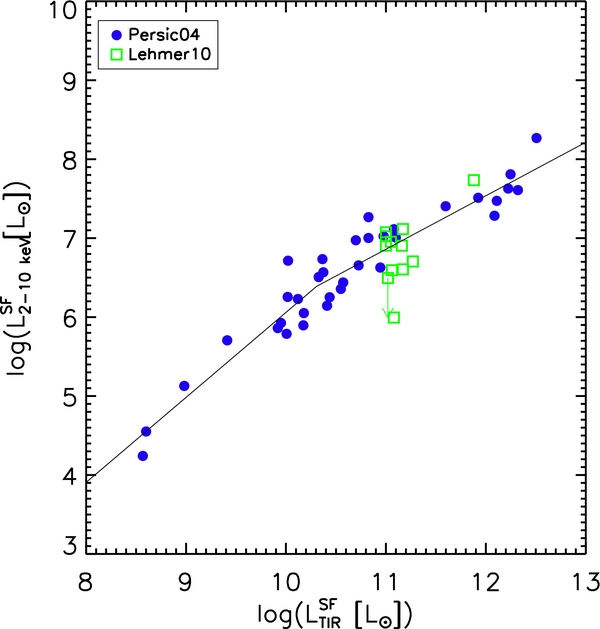
Figure 2. Relationship between IR and X-ray emission of star-forming galaxies based on the sample of Persic et al. (2004) and Lehmer et al. (2010; see Equation (13)).
Download figure:
Standard image High-resolution image3.4. SMBH SED Template
The grand unified model of AGNs (Antonucci 1993) states that all AGNs are intrinsically the same and the emerging SED is only determined by the line of sight with respect to the dusty torus; the type 2 objects are the obscured version of the type 1 objects. Adopting this scenario, we first constructed the intrinsic AGN SED from type 1 data set and then modified it with extinction as characterized by the H i column density ( ) to obtain the extinction-dependent SED. A reflected component in the X-ray is always added:
where fAGN observedν is the observed SED of AGNs, fAGN intrinsicν is the intrinsic SED before extinction, and  is the extinction curve.
The significant difference from the SF SED templates is that we only used the mean SMBH SED but did not consider its dispersion. This is partly to keep computations manageable but also because of the lack of studies that fully address the dispersion of the AGN SED from the X-ray all the way to the submillimeter as a function of the BH luminosity (Hao et al. 2012).
3.4.1. The IR/Submillimeter SED of Unobscured AGNs
The distinct IR continuum feature of the unobscured AGN is strong emission of dust heated to near the sublimation temperature (∼1000 K) by UV/optical radiation from the accretion disk. This feature serves as the basis of various mid-IR AGN selection techniques (Lacy et al. 2004; Stern et al. 2005; Armus et al. 2007; Donley et al. 2008; Wu et al. 2011). The shape of this feature has been well characterized with the emission peaking at 3–5 μm and the 1–30 μm slope α = 1 ± 0.3 (fν ∝ ν−α), although the slope estimate depends on the definition of the photometric bands and their placement with respect to the silicate feature besides the intrinsic dispersion. Generally, the broadband photometric observations indicate slopes between 1.0 and 1.5 (e.g., Neugebauer et al. 1987; Haas et al. 2003). The Spitzer Infrared Spectrograph (IRS) observations of a large sample of local AGNs reveal smaller slopes for the continuum underlying the silicate feature. For example, the whole sample of 87 PG quasars shows a relatively universal slope with median and standard deviations of α5–30 μm = 0.75 ± 0.35 (fν ∝ ν−α) (Shi et al. 2007; also see Netzer et al. 2007; Maiolino et al. 2007). The Seyfert 1 objects in the complete 12 μm sample have α15–30 μm = 0.85 ± 0.61 (Wu et al. 2009) where the slightly steeper slope and the larger dispersion are likely caused by the larger SF contamination in these low-luminosity AGNs. No obvious evidence has been found in the above studies for the dependence of the slope on the BH luminosity.
The most prominent spectral feature of the unobscured AGN SED is the silicate emission features at 9.7 and 18 μm as established unambiguously by Spitzer observations (e.g., Hao et al. 2005; Shi et al. 2006). It is important to include this feature in the SED template for our model as it can affect the broadband photometry. The strength of this feature depends weakly on the SMBH luminosity (Maiolino et al. 2007), with only a factor-of-two increase for an SMBH luminosity range of 104. We thus adopt the same feature strength independent of the SMBH luminosity.
The most uncertain part of the SMBH IR SED lies above ∼30 μm where the SF emission becomes important or even dominates for quasars. One solution is to spatially separate the nuclear emission from SF regions in host galaxies; such observations are only feasible below 30 μm (e.g., Gandhi et al. 2009). Another challenging problem with this strategy is that we have no idea if the dusty torus itself is experiencing SF and how important that is. The current approach is to scale the SF with the observed aromatic feature and then subtract it off (e.g., Shi et al. 2007; Netzer et al. 2007). This leads to the conclusion that above ∼100 μm, all the observed emission typically comes from SF, and that the SED part then relies on the extrapolation from the short wavelength. In spite of significant caveats associated with the AGN SED above 30 μm, its effect on our model is limited. This is because the majority (90%) of the AGN IR emission (3–1000 μm) emerges below 30 μm; their far-IR contribution is negligible to the observed far-IR radiation.
In practice, we constructed the unobscured IR SED based on Spitzer observations of the whole PG sample that is selected based on the UV excess and are thus type 1 objects with little obscuration (Green et al. 1986). To construct the intrinsic SED, we first derived the median composite spectrum of Spitzer/IRS spectra (5–30 μm) and MIPS photometry (24, 70, and 160 μm) of all of the PG objects. With the composite spectrum, we measured the 11.3 μm aromatic feature and scaled it to derive the star-forming emission at the Spitzer wavelength based on the DH02 template. The SF emission contributes less than 15% at <30 μm and reaches ∼50% in the 70 μm filter while dominating the 160 μm filter emission. A continuous IR SED template is then constructed based on the SF-subtracted IRS spectrum and photometry in the 70 μm filter where all the aromatic features are also carefully removed. To fill the gap in the SED beyond 30 μm, as shown in Figure 3, the underlying continuum of the silicate feature is fitted with a double power law (purple dotted line) to the 5–8 μm IRS part and MIPS 70 μm photometry where the power-law index at long wavelengths is fixed to be 4 to mimic the modified blackbody with emissivity of 1.0 (νfν ∝ν4). A single power law connecting the IRS 30 μm emission and MIPS 70 μm photometry (dashed red line) is used to model the silicate emission between 30 and 38 μm. The resulting IR SED is quite consistent with the photometry-based SED derived from the Sloan Digital Sky Survey (SDSS) quasars by Richards et al. (2006), except for the much better characterized silicate features in our template.

Figure 3. IR spectrum of type 1 AGNs based on the Spitzer/IRS spectrum and MIPS photometry of PG quasars (the upper bound of the gray area). First, the median IR SED is measured for the whole PG sample. The star formation contribution is subtracted based on the measured aromatic features of this median spectrum. The solid black line and filled circles are the IRS spectrum and MIPS 70 μm photometry after subtractions. Note that the observed MIPS 160 μm is dominated by star formation. The dotted purple line describes the underlying continuum of the silicate features. It is a fit to the 5–8 μm IRS spectrum and 70 μm photometry with two power laws where the index at long wavelength is fixed to be 4 to mimic the modified blackbody emissivity of 1.0 (νfν ∝ ν4). A single power law (red dashed line) connecting the IRS 30 μm emission and MIPS 70 μm photometry is used to model the silicate emission above the continuum roughly between 30 μm and 38 μm.
Download figure:
Standard image High-resolution imageExtracting the intrinsic IR SED for a large sample of AGNs with a range of host galaxy contamination, extinctions, etc. would be quite difficult. Moreover, the spatial and spectral resolution data are not available to allow for a result comparable to that for star-forming galaxies with well characterized mean SED and associated scatter as a function of the luminosity (Dale & Helou 2002; Chapman et al. 2003). We thus adopt the mean PG quasar IR SED with no luminosity dependence or scatter. The recent work by Mullaney et al. (2011) claimed a luminosity dependence of the AGN intrinsic mid-IR/far-IR ratio in a small AGN sample. However, their low- and high-luminosity sub-samples have completely different extinctions, which could easily induce such a dependence. The studies of X-ray AGNs in the COSMOS field show no apparent luminosity and redshift dependence for their SED (Hao et al. 2012).
3.4.2. X-Ray SED As a Function of 

For the X-ray SED as a function of the H i column density, we basically adopted the work of Gilli et al. (2007). Since no scatter is included for the IR part in our model, we did not consider the scatter in the X-ray spectral slope either. While Gilli et al. (2007) argued that the scatter in the X-ray spectra is important to constrain the Compton-thick AGN population, this will not be the case for our model due to the fundamental difference in the way that the Compton-thick AGN abundance is constrained. Their CXB model derived the Compton-thick AGN by subtracting the Compton-thin AGN contribution to the CXB spectrum around 30 keV. The extrapolation of the Compton-thin AGN contribution from <10 keV to 30 keV certainly depends critically on the scatter of the power-law slope. Our model constrains the Compton-thick AGN through mid-IR data, which depends on the SMBH IR/X-ray relationship. The additional difference between their work and this study is that we included the reflected component for the quasars (e.g., Piconcelli et al. 2010). A summary is given as follows.
- 1.The unobscured SMBH SED is composed of three components, a primary power law with a cutoff at high (>100 keV) energies, a reflected component and iron 6.4 keV emission line. The power-law component arises directly from the hot corona above the accretion disk. Its shape is characterized by a photon index of Γ = 1.9 (Nandra & Pounds 1994; Reeves & Turner 2000; Piconcelli et al. 2005; Mainieri et al. 2007) and a cutoff energy of 300 keV (Molina et al. 2006; Dadina 2008). For the latter, the uncertainty is still important. This component can be reflected off the far side of the accretion disk or dusty torus, hardening the emerging radiation. The reflected component depends on the incident spectrum slope and the observed inclination. It is modeled for Γ = 1.9 and the relative normalization is fixed to be 1.3, which is the average for type 1 lines of sight assuming a torus half-opening angle of 45°. The iron line is assumed to have a Gaussian profile with a width of 0.4 keV and an EW of 280 eV.
- 2.For the obscured Compton-thin AGN, the intrinsic power law is the same as that for the unobscured one but the reflected component normalization is reduced to 0.88 given different viewing angles toward obscured nuclei. The extinction curve is the photoelectric absorption at solar abundances as characterized by Morrison & McCammon (1983). In total, we adopt = [21.5, 22.5, 23.5] to sample the Compton-thin X-ray SEDs.
- 3.For Compton-thick AGNs with < 1025 cm−2, the intrinsic power law is the same as that for the unobscured one while the normalization of the reflected component is fixed at 0.37. The extinction curve needs to consider the non-relativistic Compton scattering as modeled through the code of Yaqoob (1997).
- 4.For Compton-thick AGNs with > 1025 cm−2, all transmitted photons are down-scattered by Compton recoil and only the reflected component is visible.


The relative normalization of the X-ray spectrum with respect to the IR part is derived through the modified version of the tight relationship between the 2–10 keV and 12.3 μm luminosities for 22 Seyfert galaxies in Gandhi et al. (2009). These galaxies are well resolved at 12.3 μm so that SF can be removed reliably. Galaxies in that work are a mix of Seyfert 1, Seyfert 2, and Compton-thick AGNs, while what we need here is the relationship only for type 1 AGNs, specifically PG quasars. At 12.3 μm, the silicate emission feature can be important. As shown in Figure 4, we thus modify the Gandhi et al. (2009) relationship by keeping the slope but modifying the normalization to produce the median X-ray/12.3 μm ratio of 34 PG quasars whose X-ray and IR data are derived from Cappi et al. (2006) and Shi et al. (2007), respectively. For these PG objects, the contribution from SF to the 12.3 μm emission is negligible as evidenced by the extreme low aromatic feature equivalent width (EW11.3 μm PAH ≲ 0.05 μm). The derived relationship is
where L2–10 keV and L12.3 μm are unobscured 2–10 keV and 12.3 μm luminosities, respectively. To evaluate the effect of this scatter on the model, we explored two additional variants of the model with the normalizations 0.2 dex higher and lower, respectively, where 0.2 dex is the 3σ dispersion of the mean ratio of the PG objects.
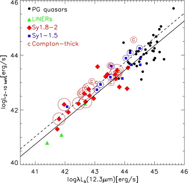
Figure 4. Relationship between 2 and 10 keV unobscured X-ray and 12.3 μm luminosities. The dashed line is the best fit for all Seyfert and LINER galaxies with well-resolved images at 12.3 μm (circled symbols; Gandhi et al. 2009). The solid line is the fit adopted in this paper that is exclusively for PG quasars. It is derived by fixing the slope as that for Seyfert and LINER ones but recalculating the normalization to produce the median trend of PG quasars. The offset between the dashed and solid lines is due to the strong silicate features in the PG quasars.
Download figure:
Standard image High-resolution image3.4.3. H i Column Density Distribution
The H i column density distribution is key to understanding AGN physics and the CXB. Its proper characterization requires unbiased sample selections and secure measurements of H i column densities. In the local universe, optically selected samples offer the least bias compared to UV/X-ray (biased against heavily extinguished objects and low-luminosity AGNs) and IR (biased against unobscured objects and low-luminosity AGNs). Maiolino & Rieke (1995) have attempted to compile all Seyfert galaxies at mB < 13.4. The Seyfert 2 to Seyfert 1 ratio is found to be as high as 4:1. This ratio is consistent with that found in the Palomar nuclear spectroscopic survey of local galaxies at mB < 12.5 (Ho et al. 1997). Both studies dealt carefully with host galaxy light dilution and the result should be quite reliable. Both studies probed very low luminosity AGNs with bolometric luminosities around 109 L☉. Hao et al. (2005) instead found 1:1 for the Seyfert 2/Seyfert 1 ratio around Lbol ∼ 109L☉ and decreasing toward higher luminosities. The discrepancy can be partly due to the luminosity dependence but also that the SDSS spectra in Hao et al. (2005) with large aperture and relatively low quality suffer significant host dilution. By building a Seyfert 2 sample from Maiolino & Rieke (1995) and Ho et al. (1997), Risaliti et al. (1999) measured the H i column density distribution. Combining this with works of Cappi et al. (2006) for Seyfert 1 galaxies, we characterized the column density distribution with three bins:
where  is the probability per logarithm of the H i
column density and the unobscured AGN fraction ftype-1 is defined as the number of objects with
is the probability per logarithm of the H i
column density and the unobscured AGN fraction ftype-1 is defined as the number of objects with  < 22 to the total, while fCT is defined to be the fraction of CT (
 > 24) among the obscured AGNs (22 <
  < 26).
Beyond the local universe, it is increasingly difficult to measure the H i column density distribution directly. Our model thus allows both luminosity and redshift evolution of ftype-1 and fCT:
where f0, type-1 is fixed to be 0.2 and f0, CT is fixed to be 0.5 at LBHTIR = 109 L☉, in order to approximate the result of Maiolino & Rieke (1995), Ho et al. (1997), and Risaliti et al. (1999). We also impose a maximum and minimum fractions of 95% and 5%, respectively, for each column range (type 1, Compton-thin type 2, and Compton-thick). There are four free parameters in total to describe the H i column density distribution.
3.4.4. The UV/Optical Part of Unobscured SED
The composite UV/optical/near-IR SED is taken from Richards et al. (2006) based on the SDSS type 1 quasars. We combined this part with X-ray emission through the X-ray/optical luminosity relationship as established by Steffen et al. (2006)
where αox = −0.384log(Lν, 2500 Å/Lν, 2 keV).
3.4.5. The Extinction Curve at UV/Optical/IR Wavelength
The extinction curve for the UV/optical/IR emission is adopted to be that of the SMC from Pei (1992), which is a good approximation for reddened AGNs as discussed in Hopkins et al. (2007). To relate the amount of extinction in the optical/IR to that in the X-ray, we need to assume a gas-to-dust ratio represented by  /AV in AGNs. Studies show that in AGNs, the extinction in the optical and IR is significantly less than what is expected from the gas-to-dust ratio in the Milky Way or SMC (e.g., Risaliti et al. 2000; Maiolino et al. 2001; Shi et al. 2006). Two possible reasons are that there is a large amount of dust-free gas surrounding SMBH or that the X-ray and IR emitting sources are spatially offset so that they are not extinguished exactly by the same material. We here increased the gas-to-dust ratio by a factor of 100 to match the observed average ratio between the X-ray H i column density and the silicate absorption feature (Shi et al. 2006).
3.5. A Summary of Model Components
Our model first assumes total IR LFs that are described by a double power law with four parameters (break luminosity and density along with the faint- and bright-end slopes). The IR LF is assumed to evolve with redshift in both break luminosity and density, each of which is a polynomial function of redshift with three parameters. Therefore, the total IR LF has a total of 10 parameters. The model then introduces the SMBH energy fraction in the total IR band to decompose the emission into SMBH and star-forming components. At a given IR luminosity, the distribution of SMBH energy fractions is assumed to be a Gaussian function with both mean and scatter depending on the luminosity, while the mean is further assumed to show redshift dependence. There are five free parameters in total, including two for the redshift dependence of the mean and one for its luminosity dependence, one for the scatter at the total IR luminosity of 1012.3 L☉, and one for its luminosity dependence. The mean fraction at 1012.3 L☉ is fixed based on local ULIRG objects. For each power source (star forming and SMBH), the model then converts the emission in the total IR band to other wavelengths using star-forming and AGN SEDs. For the former, luminosity-dependent empirical SEDs are used. For the latter, H i columns are added to extinguish the type 1 empirical SEDs. H i columns are divided into three ranges representing type 1, Compton-thin type 2, and Compton-thick, which are described by two parameters to give the relative frequencies of occurrence (the sum of which needs to be normalized). Each parameter has a local value fixed at the SMBH IR luminosity of 109 L☉, and is assumed to follow a simple power-law dependence on both luminosity and redshift. Therefore the H i columns have four parameters in total. The model has a total of 19 free parameters.
4. NUMERICAL APPROACH
Our approach to constraining the model is to fit both X-ray and IR survey data, with the basic assumption that all the galaxies are experiencing both SF and nuclear accretion activities with relative intensities that vary with both redshift and luminosity. The model is composed of four components (see Section 3 for details): the total IR LF, the SMBH energy fraction in the IR, the SF SED, and SMBH SED. In principle, the combination of these four can predict any observed properties that are related to galaxy number densities and SEDs, such as number counts, redshift distributions, LFs, etc.
The model has a total of 19 free parameters. To incorporate the uncertainties on the observational constraints that we adopted for the model, we present four variants of the model as summarized in Table 1, varying the SMBH IR/X-ray ratio and redshift evolution in the SF SED. The numerical calculation starts with the generation of a multi-dimensional array of the flux density at a given filter for an object at the given total IR luminosity, SF color, redshift, SMBH energy fraction, and H i column density, i.e., fν(filter, LTIR, SF color, z, fBH,  ), where the numerical grid of each dimension is pre-defined and thus fν is fixed. Each fν has an associated total probability function (the product of four model components):

Ptot contains all free parameters whose best values will be obtained by fitting to the data. The general procedure to derive fν and Ptot is as follows.
- 1.Φ(LTIR, z) is a function of LTIR and z. The numerical grid of LTIR covers the luminosity range from 107 L☉ to 1014 L☉ with a resolution of 0.2 dex. The redshift grid starts with z = 0.001 and increases with Δz/z = 0.1 until z = 1.0 with a total of 63 bins. At z ⩾ 1.0, Δz is fixed to be 0.1 up to z = 6.
- 2.The given LTIR is divided into the SF component LSFTIR and SMBH component LBHTIR according to the SMBH energy fraction logfBH. The logfBH has a range from −6.0 to 0.0 with a resolution of 0.2 dex. At logfBH = −6.0, the SMBH contribution at any wavelength is negligible. Also, such a low value is needed to ensure the possibility of negligible SMBH radiation in a IR luminous object, i.e., L2–10 keV < 1042 erg s−1.
- 3.For the given LSFTIR, the SF SED is assigned according to all possible SF colors as defined by log (fν(IRAS60 μm)/fν(IRAS100 μm)). The SF color varies from C0−3σc to C0+3σc with a step of 0.5σc, where C0 is the function of LSFTIR (see Section 3.3.1). Each SF color has a probability of PSF color. With the assigned SF SED, the LSFν(filter) is obtained by convolving the SED with the filter curve. Note that in the X-ray, the flux is the direct integral of the SED between the edges of the band.
- 4.For a given LBHTIR, the SMBH SED is assigned according to the H i column density. The grid is defined to be logcm−2 = [0, 21.5, 22.5, 23.5, 24.5, 25.5], each of which has a probability of . The assigned SED is then used to derive the LBHν(filter).
- 5.The final luminosity in a filter is the sum of LSFν(filter) and LBHν(filter). This is divided by the distance modulus to obtain the final fν(filter).


Table 1. A Summary of Different Variants of the Model
| Models | Description | pc | LogLBH2–10 keV vs. LogLBH12 μm |
|---|---|---|---|
| (1) | (2) | (3) | (4) |
| Reference (solid line) | Reference-model | 0.0 |  |
| fast_evol_SED_SF (dashed line) | Strong evolution of SF SED | 2.0 |  |
| low_IR2X_BH (dot-dashed line) | Lower BH IR/X-ray ratio | 0.0 |  |
| high_IR2X_BH (three-dot-dashed line) | Higher BH IR/X-ray ratio | 0.0 |  |
Notes. Column 1: the names of different variants of the model. Column 2: the description to the specific variant of the model. Column 3: the pc value (Equation (12)) used to quantify the star-forming SED redshift evolution. Column 4: the SMBH X-ray vs. IR luminosity relationship used to connect the AGN X-ray SED part with the IR part. Compared to the reference model, the fast_evol_SED_SF variant assumes strong redshift evolution of the star-forming SED. The low_IR2X_BH and high_IR2X_BH variants have X-ray luminosities at given IR luminosities for the SMBH radiation 0.2 dex lower and higher, respectively. See Sections 3.3.2, 3.4.2, and 6.4. The line style for each variant of the model is used for all figures in this paper.
Download table as: ASCIITypeset image
At a given total IR luminosity and redshift, the above grids produce 2340 SEDs covering the range of the SMBH energy fraction, the extinction, and the scatter in the SF SED, with examples shown in Figure 5. In total, there are 10 million SEDs to cover the IR luminosity, redshift, the BH energy fraction, the SF SED, and the H i columns. After producing fν(filter, LTIR, SF color, z, fBH,  ), the free parameters in Ptot are derived by fitting to the observations. The fitting scheme is the Levenberg–Marquardt least-square technique with the IDL program mpfit.pro (Markwardt 2009).
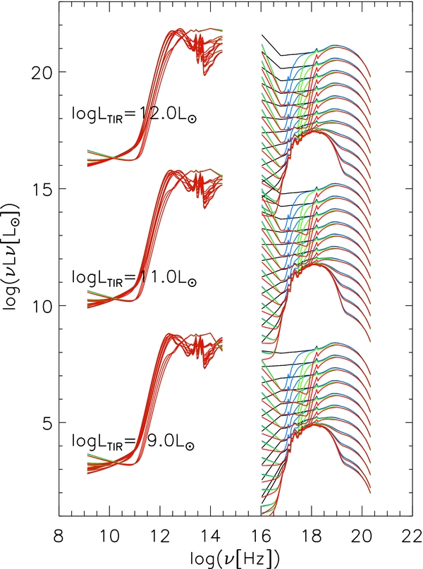
Figure 5. Examples of SEDs at three given total IR luminosities. Note that the model adopts a total of 2340 SEDs at a given total IR luminosity and a redshift that covers the range of the SMBH energy fraction, the extinction, and the scatter in the star formation SEDs. Here it shows SEDs at lower resolution grids over the above three parameters for clarity. Different colors are for different extinctions.
Download figure:
Standard image High-resolution image5. DATA FOR THE FIT
Our model fits a total of 617 data points from the local LFs plus two basic types of data from deep surveys, namely, number counts and redshift distributions. The basic information of these data sets is listed in Table 2. The main advantages of our fit strategy compared to those fitting directly to LFs at different redshifts include: (1) that we isolated the number counts as an independent data set for the fit; these are the most direct result of the deep survey observations and contain the least modeling uncertainties; and (2) that we avoided the uncertainties and systematic differences associated with the K-corrections for the LFs derived in different studies.
Table 2. Data Sets to Derive the Best-fit Parameters
| Differential Number Counts (237 Data Points) | ||||
|---|---|---|---|---|
| Band | Reference | Fields | Area (deg2) | Depth |
| 17–60 keV | Krivonos et al. (2010) | All-sky | All-sky | 7 × 10⁻¹² erg s−1 cm−2 [5σ] |
| 15–55 keV | Ajello et al. (2012) | All-sky | All-sky | 6 × 10⁻¹² erg s−1 cm−2 [5σ] |
| 4–8 keV | Lehmer et al. (2012) | CDFS | 0.13 | 4.6 × 10⁻¹⁷ erg s−1 cm−1 [Pdet >0.004] |
| 2–10 keV | Georgakakis et al. (2008) | CDF-N | 0.11 | 10−16 erg s−1 cm−2 [P <4 × 10⁻⁶] |
| CDF-S | 0.06 | 2 × 10⁻¹⁶ erg s−1 cm−2 [P <4 × 10⁻⁶] | ||
| ECDF-S | 0.25 | 3 × 10⁻¹⁶ erg s−1 cm−2 [P <4 × 10⁻⁶] | ||
| EGS | 0.63 | 3 × 10⁻¹⁶ erg s−1 cm−2 [P <4 × 10⁻⁶] | ||
| EN1 | 1.47 | 10−15 erg s−1 cm−2 [P <4 × 10⁻⁶] | ||
| XBOOTES | 9.24 | 6 × 10⁻¹⁶ erg s−1 cm−2 [P <4 × 10⁻⁶] | ||
| Ueda et al. (2005) | AMSS | 278 | 10−13 erg s−1 cm−2 [5σ] | |
| Elvis et al. (2009) | COSMOS | 0.5 | 7.3 × 10⁻¹⁶ erg s−1 cm−2 [P <2 × 10⁻⁵] | |
| Lehmer et al. (2012) | CDFS | 0.13 | 5.1 × 10⁻¹⁸ erg s−1 cm−2 [Pdet >0.004] | |
| 0.5–2 keV | Georgakakis et al. (2008) | CDF-N | 0.11 | 10−17 erg s−1 cm−2 [P <4 × 10⁻⁶] |
| CDF-S | 0.06 | 2 × 10⁻¹⁷ erg s−1 cm−2 [P <4 × 10⁻⁶] | ||
| ECDF-S | 0.25 | 3 × 10⁻¹⁷ erg s−1 cm−2 [P <4 × 10⁻⁶] | ||
| EGS | 0.63 | 3 × 10⁻¹⁷ erg s−1 cm−2 [P <4 × 10⁻⁶] | ||
| EN1 | 1.47 | 10−16 erg s−1 cm−2 [P <4 × 10⁻⁶] | ||
| XBOOTES | 9.24 | 6 × 10⁻¹⁷ erg s−1 cm−2 [P <4 × 10⁻⁶] | ||
| Elvis et al. (2009) | COSMOS | 0.5 | 1.9 × 10⁻¹⁶ erg s−1 cm−2 [P <2 × 10⁻⁵] | |
| Lehmer et al. (2012) | CDFS | 0.13 | 5.1 × 10⁻¹⁸ erg s−1 cm−2 [Pdet >0.004] | |
| Spitzer 24 μm | Béthermin et al. (2010) | FIDEL ECDF-S | 0.23 | 60 μJy [80% complete] |
| FIDEL EGS | 0.41 | 76 μJy [80% complete] | ||
| COSMOS | 2.73 | 96 μJy [80% complete] | ||
| SWIRE LH | 10.04 | 282 μJy [80% complete] | ||
| SWIRE EN1 | 9.98 | 261 μJy [80% complete] | ||
| SWIRE EN2 | 5.36 | 267 μJy [80% complete] | ||
| SWIRE ES1 | 7.45 | 411 μJy [80% complete] | ||
| SWIRE CDFS | 8.42 | 281 μJy [80% complete] | ||
| SWIRE XMM | 8.93 | 351 μJy [80% complete] | ||
| IRAS 25 μm | Hacking & Soifer (1991) | All-sky | All-sky | 300 mJy [5σ] |
| Spitzer 70 μm | Béthermin et al. (2010) | FIDEL ECDF-S | 0.19 | 4.6 mJy [80% complete] |
| COSMOS | 2.41 | 7.9 mJy [80% complete] | ||
| SWIRE LH | 11.88 | 25.4 mJy [80% complete] | ||
| SWIRE EN1 | 9.98 | 14.7 mJy [80% complete] | ||
| SWIRE EN2 | 5.34 | 26.0 mJy [80% complete] | ||
| SWIRE ES1 | 7.43 | 36.4 mJy [80% complete] | ||
| SWIRE CDFS | 8.28 | 24.7 mJy [80% complete] | ||
| Spitzer 160 μm | Béthermin et al. (2010) | FIDEL EGS | 0.38 | 45 mJy [80% complete] |
| COSMOS | 2.58 | 46 mJy [80% complete] | ||
| SWIRE LH | 11.10 | 92 mJy [80% complete] | ||
| SWIRE EN1 | 9.30 | 94 mJy [80% complete] | ||
| SWIRE EN2 | 4.98 | 90 mJy [80% complete] | ||
| SWIRE ES1 | 6.71 | 130 mJy [80% complete] | ||
| SWIRE CDFS | 7.87 | 88 mJy [80% complete] | ||
| Herschel 100 μm | Berta et al. (2011) | GOODS-N | 0.083 | 3.0 mJy [3σ] |
| GOODS-S | 0.083 | 1.2 mJy [3σ] | ||
| LH | 0.18 | 3.6 mJy [3σ] | ||
| COSMOS | 2.04 | 9.0 mJy [3σ] | ||
| Herschel 160 μm | Berta et al. (2011) | GOODS-N | 0.083 | 5.7 mJy [3σ] |
| GOODS-S | 0.083 | 2.4 mJy [3σ] | ||
| LH | 0.18 | 7.5 mJy [3σ] | ||
| COSMOS | 2.04 | 10.2 mJy [3σ] | ||
| Herschel 250 μm | Oliver et al. (2010) | A2218 | 0.0225 | 13.8 mJy [50% complete] |
| FLS | 5.81 | 17.5 mJy [50% complete] | ||
| Lockman-North | 0.34 | 13.7 mJy [50% complete] | ||
| Lockman-SWIRE | 13.20 | 25.7 mJy [50% complete] | ||
| GOODS-N | 0.25 | 12.0 mJy [50% complete] | ||
| Herschel 350 μm | Oliver et al. (2010) | A2218 | 0.0225 | 16.0 mJy [50% complete] |
| FLS | 5.81 | 18.9 mJy [50% complete] | ||
| Lockman-North | 0.34 | 16.5 mJy [50% complete] | ||
| Lockman-SWIRE | 13.20 | 27.5 mJy [50% complete] | ||
| GOODS-N | 0.25 | 13.7 mJy [50% complete] | ||
| Herschel 500 μm | Oliver et al. (2010) | A2218 | 0.0225 | 15.1 mJy [50% complete] |
| FLS | 5.81 | 21.4 mJy [50% complete] | ||
| Lockman-North | 0.34 | 16.0 mJy [50% complete] | ||
| Lockman-SWIRE | 13.20 | 33.4 mJy [50% complete] | ||
| GOODS-N | 0.25 | 12.8 mJy [50% complete] | ||
| SCUBA 850 μm | Borys et al. (2003) | HDF-N | 0.046 | ∼3 mJy [1σ] |
| Coppin et al. (2006) | SHADES | 0.20 | ∼2 mJy [1σ] | |
| Aztec 1100 μm | Scott et al. (2012) | GOODS-N, LH, GOODS-S, ADF-S, SXDF | 1.6 | 0.4–1.7 mJy [1σ] |
| Hatsukade et al. (2011) | ADF-S | 0.25 | ∼0.5 mJy [1σ] | |
| Mambo 1200 μm | Greve et al. (2004) | EN2, LH | 0.10 | 0.6 mJy [1σ] |
| Lindner et al. (2011) | LH-N | 0.16 | 0.75 mJy [1σ] | |
| Redshift Distributions (174 Data Points) | ||||
| Bands | Fields | Spec-z | All-z | Reference |
| 2–10 keV | CDF-N | 61% | 87% | Barger et al. (2005), Donley et al. (2007) |
| Trouille et al. (2008) | ||||
| COSMOS | 60% | 98% | Civano et al. (2012) | |
| CDF-S | 51% | 97% | Luo et al. (2010) | |
| ECDF-S | 64% | 95% | Silverman et al. (2010) | |
| XMS | 87% | 87% | Barcons et al. (2007) | |
| 0.5–2 keV | CDF-N | 63% | 86% | Barger et al. (2005), Donley et al. (2007) |
| Trouille et al. (2008) | ||||
| COSMOS | 59% | 98% | Civano et al. (2012) | |
| CDF-S | 50% | 97% | Luo et al. (2010) | |
| ROSAT-NEP | 97% | 97% | Henry et al. (2006) | |
| ROSAT-RIXOS | 93% | 93% | Mason et al. (2000) | |
| Spitzer 24 μm | COSMOS | 0% | 100% | Le Floc'h et al. (2009) |
| GOODS-S | 90% | 90% | Barger et al. (2008) | |
| 5MUSES | 98% | 98% | Wu et al. (2010) | |
| IRAS 60 μm | All Sky | 100% | 100% | Sanders et al. (2003) |
| SCUBA 850 μm | Seven fields | 75% | 75% | Chapman et al. (2005) |
| Aztec 1100 μm | COSMOS | 41% | 100% | Smolcic et al. (2012) |
| Local Luminosity Functions (37 Data Points) | ||||
| Bands | Reference | |||
| 15–55 keV | Ajello et al. (2012) | |||
| 2–10 keV | Ueda et al. (2011) | |||
| IRAS 12 μm | Rush et al. (1993) | |||
| IRAS 25 μm | Shupe et al. (1998) | |||
While a large number of data sets is available in the literature, we generally preferred those with good statistics. We thus included either those based on the combined fields or individual results of fields with either large areas or high sensitivities. We also avoid double fitting data sets of the same field that were from different authors or papers. Overall, the number counts include X-ray data at 17–60 keV, 15–55 keV, 2–10 keV, and 0.5–2 keV bands, and IR/submillimeter data ranging from 24 μm to 1200 μm. The redshift distributions also cover a range of wavelengths, field areas, and limiting flux cuts. For the same field, the redshift distributions with different flux cuts offer constraints on the model LFs in the different luminosity and redshift ranges. The redshift completeness in data sets we used is high, >90%, either from spec-z, photo-z, or both. The error bars include Poisson noise and cosmic variances with the latter estimated by a two-point correlation function from direct observations or the cosmological model of Trenti & Stiavelli (2008). Except for a few data sets with high flux cuts, photo-z measurements always constitute an important fraction, especially at z > 1. For X-ray sources, photo-z errors can be significant due to the faint optical/near-IR counterparts along with the power-law featureless shape. We thus added additional errors to redshift distributions for the photo-z part through the simple bootstrapping method.
5.1. Number Counts
5.1.1. X-Ray Number Counts
All sky surveys in the 17–60 keV by International Gamma-Ray Astrophysics Laboratory (Krivonos et al. 2010) and 15–55 keV by Swift (Ajello et al. 2012) probe bright AGNs down to 6–7 × 10⁻¹² erg s−1 cm−2, whose number counts offer useful constraints on the model's behavior in the local universe. The Chandra deep survey data are used to probe high-z universe. Georgakakis et al. (2008) combined several surveys including the CDF-N/S, ECDF-S, EGS, EN1, and XBOOTES fields, to offer number counts in 0.5–2 and 2–10 keV with high signal-to-noise ratio across a large flux range. It reaches 1.0 × 10⁻¹⁷ and 1.0 × 10⁻¹⁶ erg s−1 cm−2 in two bands, respectively. Although galactic stars are not removed in this work, their contributions are small (<10%; Bauer et al. 2004). The additional data in the COSMOS field by Elvis et al. (2009) are also included for the fit. The recent 4 Ms CDFS data from Lehmer et al. (2012) are further used to probe number counts at the faintest end, for which 4–8 keV data along with 0.5–2 keV and 2–10 keV are all included. An additional large-area ASCA survey in the 2–10 keV is also included (Ueda et al. 2005). The small difference (∼1%) in the counts between two different galactic latitudes of this survey indicates a small contribution from Galactic contaminators. The published errors of the number counts in the above studies have taken into account Poisson noises and cosmic variances. If a fixed Photon index (e.g., 1.4) is used to convert the count rate to the flux, we added an additional uncertainty of 0.1 dex quadratically.
5.1.2. Spitzer Number Counts
We fitted to the Spitzer number counts at 24, 70, and 160 μm measured by Béthermin et al. (2010), which are generally consistent with previous works (Papovich et al. 2004; Shupe et al. 2008; Le Floc'h et al. 2009; Frayer et al. 2009). The study incorporates data from fields including SWIRE, COSMOS, and FIDEL. Besides standard data reduction and photometry measurements, the incompleteness and Eddington bias are also corrected in that work, with further removal of stars. The counts reach 35 μJy, 3.5 mJy, and 40 mJy at 24, 70, and 160 μm, respectively. Their stacking data at two longer wavelengths are not used in the fits but are plotted for illustration. At 24 μm, we added the IRAS 25 μm data from Hacking & Soifer (1991) by assuming a flat SED in νfν, which provides constraints in the local universe.
5.1.3. IRAS Number Counts
In addition to the IRAS 25 μm number counts, the counts at 60 μm from Lonsdale et al. (1990) are also included to provide constraints at the brightest flux end (i.e., local universe). The error is caused by the large-scale structure of the local universe. We estimated it roughly as the difference in the number counts between the south and north Galactic cap.
5.1.4. Herschel Number Counts
Our fit includes the number counts at 250, 350, and 500 μm of detected sources in the HerMES field as estimated by Oliver et al. (2010). The depth reaches around 15 mJy at three wavelengths. Their published uncertainties account for Poisson noises, cosmic variances, and uncertainties associated with flux measurements and incompleteness corrections. Deeper counts obtained through P(D) (probability of deflection) analysis of the same field (Glenn et al. 2010) are included only for illustration. At 100 and 160 μm, we adopted the result of Berta et al. (2011) from three fields (COSMOS, Lockman Hole, and GOODS-N). The data reach down to 2.0 mJy at 100 μm and 5 mJy at 160 μm. The estimated errors on the counts include Poisson noise and field-to-field variations.
5.1.5. SCUBA/Aztec/Mambo Submillimeter Number Counts
The SCUBA counts at 850 μm are collected from Borys et al. (2003) and Coppin et al. (2006) with the overall flux range from 2.5 to 25 mJy. The Aztec number counts at 1.1 mm are from two recent studies, Hatsukade et al. (2011) and Scott et al. (2012). The combined counts cover the flux range from about 0.5 to 10 mJy. The Mambo 1.2 mm counts are from Greve et al. (2004) and Lindner et al. (2011).
5.2. Redshift Distributions
5.2.1. X-Ray Redshift Distributions
For 503 objects in the Chandra CDF-N 2 Ms catalog (Alexander et al. 2003), the redshift measurements are compiled from Barger et al. (2005), Donley et al. (2007), and Trouille et al. (2008). In the hard X-ray band, we constructed two redshift distributions above limiting fluxes 3 × 10⁻¹⁶ and 3 × 10⁻¹⁵ erg s−1 cm−2, respectively, and in the soft band (0.5–2 keV) above two limiting fluxes of 6 × 10⁻¹⁶ and 6 × 10⁻¹⁷ erg s−1 cm−2. For each band, the first flux is near the detection limit and the second one is about 10 times brighter. The spectroscopic redshift and all redshift (spec-z+photo-z) completeness is around 65% and 90%, respectively.
For 462 sources in the Chandra CDF-S 2Ms catalog (Luo et al. 2008), the redshift measurements are available in Luo et al. (2010). Two redshift distributions in the hard X-ray are measured above 3.0 × 10⁻¹⁶ and 3.0 × 10⁻¹⁵ erg s−1 cm−2, respectively. In the soft band, the limiting fluxes of 5.0 × 10⁻¹⁷ and 5.0 × 10⁻¹⁶ erg s−1 cm−2 are used. The spec-z and all redshift completeness is around 55% and 97%, respectively.
With deep multiple optical/near-IR follow-ups, virtually all 1761 X-ray AGNs in the COSMOS field are identified (Civano et al. 2012). The redshift distribution above 3 × 10⁻¹⁵ erg s−1 cm−2 in 2–10 keV and 6 × 10⁻¹⁶ erg s−1 cm−2 in 0.5–2 keV are used for the fit, with spec-z and all redshift completeness reaching 60% and 98%, respectively.
The extended CDF-S (ECDF-S) contains a total of 762 sources (Lehmer et al. 2005). The redshift distribution in 2–10 keV is constructed at >2.0 × 10⁻¹⁵ erg s−1 cm−2 (Silverman et al. 2010). The spec-z and all redshift completeness is 64% and 95%, respectively. The XMS offers 318 X-ray sources at bright fluxes (≳×10−14 erg s−1 cm−2) with high optical identification (90%; Barcons et al. 2007). The redshift distribution is constructed above the 2–10 keV flux of 5 × 10⁻¹⁴ erg s−1 cm−2 with high spectroscopic completeness (87%).
In the soft band, two additional surveys by the ROSAT are included. Henry et al. (2006) have defined a statistical sample above 2 × 10⁻¹⁴ erg s−1 cm−2 from the ROSAT north ecliptic pole survey. The spectroscopic redshifts are highly complete (>95%; Gioia et al. 2003). We have measured the redshift distribution above 5 × 10⁻¹⁴ erg s−1 cm−2 from this sample. The second one above 3 × 10⁻¹⁴ erg s−1 cm−2 is constructed from the ROSAT-RIXOS survey (Mason et al. 2000). Note that for these two surveys with high limiting fluxes, the galactic stars are identified and removed.
5.2.2. IR/Submillimeter Redshift Distributions
In the COSMOS field, Le Floc'h et al. (2009) measured redshift distributions of 24 μm sources. Here we included two measurements with flux limits of 0.08 and 0.15 mJy, respectively. The one with the highest flux limit (0.3 mJy) is not used since the bright sources excluded from that study may affect the distribution at z < 1. The photo-z completeness reaches 94%. In GOODS-N, Barger et al. (2008) carried out a highly complete spec-z survey. At f24 μm > 0.3 mJy, we measured the redshift distribution with spec-z completeness of 90%. From the Spitzer 5MUSES data (Helou et al. 2013, in preparation), we measured the redshift distribution of 24 μm sources at f24 μm > 5 mJy, where the spec-z completeness reaches 98%. At 60 μm in the local universe, the spec-z distribution of the IRAS RBGS sample is included (Sanders et al. 2003).
Chapman et al. (2005) carried out a spec-z survey of submillimeter sources at 850 μm and modeled the redshift distribution for f850 μm > 5 mJy. We fitted this distribution in our study. We further included the redshift distribution of sources at Aztec 1100 μm as measured by Smolcic et al. (2012) where the spec-z and redshift completeness are roughly 41% and 100%, respectively.
5.3. Local LFs
6. DATA FITTING RESULTS
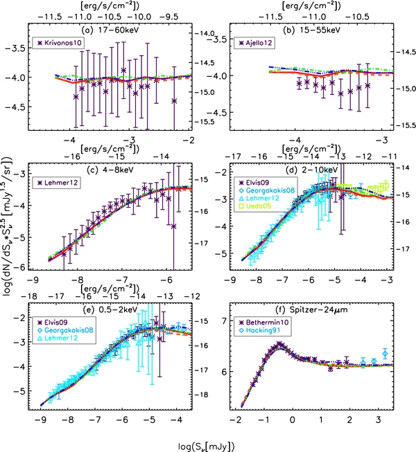
The fits to the number counts, redshift distribution, and local LFs are shown in Figures 6–8, respectively, along with the best-fit parameters in Table 3 for four variants of the model. The model fits 617 data points in total, with 371, 195, and 51 points from number counts, redshift distributions, and local LFs, respectively. Overall our model reproduces the observations reasonably well. The differences between the fits and data appear at some data points but are generally smaller than 0.2 dex or within 2σ. Cosmic variances or photo-z errors are significant for some of these deviations. The reduced χ2 of four variants of the model ranges from 2.7 to 2.9, with at least 0.75 contributed by caveats associated with data themselves (see Section 6.4 for details). In the following, we go through each version of the model and point out the differences between the fit and the data and their causes, if possible.
Download figure:
Standard image High-resolution image
Download figure:
Standard image High-resolution image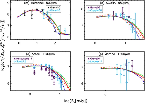
Figure 6. Fit data set I: number counts. All symbols are the observations while those in the black are not used for the fitting. The four variants of the model are shown with different line styles: solid line for reference variant, dashed line for fast_evol_SED_SF, dot-dashed line for low_IR2X_BH, and triple-dot-dashed line for high_IR2X_BH. The reference model is the one with the minimum χ2. The fast_evol_SED_SF variant assumes strong redshift evolution of the star-forming SED. The low_IR2X_BH and high_IR2X_BH variants have X-ray luminosities at given IR luminosities for the SMBH radiation 0.2 dex lower and higher, respectively (see Table 1).
Download figure:
Standard image High-resolution image
Download figure:
Standard image High-resolution image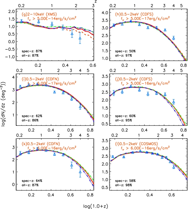
Download figure:
Standard image High-resolution image
Download figure:
Standard image High-resolution image
Figure 7. Fit data set II: redshift distribution. All symbols are the observations. The four variants of the model are shown with different line styles: solid line for reference variant, dashed line for fast_evol_SED_SF, dot-dashed line for low_IR2X_BH, and triple-dot-dashed line for high_IR2X_BH (see Table 1).
Download figure:
Standard image High-resolution image
Figure 8. Fit data set III: local IRAS and X-ray luminosity functions. All symbols are the observations. The four variants of the model are shown with different line styles: solid line for reference variant, dashed line for fast_evol_SED_SF, dot-dashed line for low_IR2X_BH, and triple-dot-dashed line for high_IR2X_BH (see Table 1).
Download figure:
Standard image High-resolution imageTable 3. The Best-fit Parameters
| Parameter | Reference | fast_evol_SED_SF | low_IR2X_BH | high_IR2X_BH |
|---|---|---|---|---|
| (1) | (2) | (3) | (4) | (5) |
| The total IR LF | ||||
| logL*, 0(LogL☉) | 10.61 ± 0.04 | 10.67 ± 0.04 | 10.60 ± 0.04 | 10.62 ± 0.04 |
| k1, l | 0.35 ± 0.40 | 1.65 ± 0.37 | 1.65 ± 0.36 | 0.81 ± 0.39 |
| k2, l | 15.33 ± 1.63 | 6.97 ± 1.50 | 9.70 ± 1.46 | 13.00 ± 1.57 |
| k3, l | −15.19 ± 1.76 | −7.64 ± 1.63 | −9.32 ± 1.60 | −12.95 ± 1.70 |
| logΦ*, 0(Mpc−3LogL−1☉) | −2.67 ± 0.06 | −2.71 ± 0.06 | −2.64 ± 0.06 | −2.66 ± 0.06 |
| k1, d | 3.68 ± 0.57 | 2.96 ± 0.57 | 2.57 ± 0.53 | 2.80 ± 0.56 |
| k2, d | −16.25 ± 2.24 | −10.90 ± 2.25 | −11.70 ± 2.03 | −12.12 ± 2.21 |
| k3, d | 9.39 ± 2.36 | 3.61 ± 2.42 | 4.77 ± 2.12 | 5.33 ± 2.34 |
| γ1 | 0.39 ± 0.03 | 0.40 ± 0.03 | 0.38 ± 0.03 | 0.36 ± 0.03 |
| γ2 | 2.49 ± 0.04 | 2.65 ± 0.05 | 2.52 ± 0.05 | 2.52 ± 0.04 |
| BH energy fraction in the total IR band | ||||
| σBH0 | 0.64 ± 0.03 | 0.75 ± 0.05 | 0.55 ± 0.02 | 0.63 ± 0.02 |
| kBH1, d | −3.33 ± 0.27 | −3.97 ± 0.32 | −3.29 ± 0.22 | −3.15 ± 0.08 |
| kBH2, d | 3.05 ± 0.44 | 6.02 ± 0.52 | 2.89 ± 0.40 | 2.87 ± 0.11 |
 |
0.74 ± 0.08 | 0.78 ± 0.08 | 0.67 ± 0.07 | 1.14 ± 0.01 |
| pσ | −0.19 ± 0.05 | −0.13 ± 0.05 | −0.09 ± 0.05 | −0.46 ± 0.01 |
| H i column density | ||||
| βz, type-1 | 1.23 ± 0.18 | 0.79 ± 0.17 | 0.91 ± 0.17 | 0.68 ± 0.13 |
| βl, type-1 | −0.66 ± 0.06 | −0.48 ± 0.06 | −0.48 ± 0.07 | −0.42 ± 0.05 |
| βz, CT | −0.79 ± 0.09 | −1.00 ± 0.09 | −1.36 ± 0.13 | −0.81 ± 0.08 |
| βl, CT | 0.44 ± 0.08 | 0.41 ± 0.07 | 0.73 ± 0.12 | 0.21 ± 0.05 |
| dof | 598 | 598 | 598 | 598 |
| χ2 | 1675.7 | 1752.8 | 1702.6 | 1608.1 |
Notes. The best-fit parameters are listed for four variants of the model (see Table 1).
Download table as: ASCIITypeset image
6.1. Fitting Number Counts
For the reference model (the solid line), the differences between the data and the fit include 0.1 dex constant overfits of the 15–55 keV number counts, 0.2–0.3 dex underfits of the 2–10 keV counts at the bright end, the 0.2 dex underfits around 0.5–2 keV fluxes from 1.5 to 4.0 × 10⁻¹⁷ erg s−1 cm−2, 0.1–0.2 dex underfits around the peak 24 μm count in the flux density range of 0.2–0.5 mJy, 0.2 dex underfits and overfits at the 70 μm bright and faint ends, respectively. Unlike the 15–55 keV counts, the 17–60 keV ones are well produced by our model so that the discrepancy seen in 15–55 keV can be due to subtle differences in the X-ray SED around the range of 15–17 keV and 55–60 keV. It is yet interesting to note that, similar to ours, several other models (Gilli et al. 2007; Treister et al. 2009; Draper & Ballantyne 2010) overproduce the 15–55 keV counts by 0.1–0.2 dex, while their adopted SEDs are not exactly the same. The difference seen at the bright end of the 2–10 keV counts is likely caused by contamination of galaxy clusters in the data (Gilli et al. 1999). In 0.5–2 keV counts, the data clearly show a transition flux (3 × 10⁻¹⁷ erg s−1 cm−2) below which normal galaxies other than AGNs start to dominate, causing the counts to go above the simple power-law extrapolation from the higher fluxes (Bauer et al. 2004; Lehmer et al. 2012), while the model also produces a similar feature but at fluxes ∼3 times lower. For the 24 μm peak counts, although the highest observed point is the result of the SWIRE data near the detection limit (Béthermin et al. 2010), the differences are seen over several adjacent data points. Since this peak is caused by aromatic features moving into the 24 μm filter around z = 1, a possible explanation is that z ∼ 1 star-forming galaxies have slightly increased aromatic-feature EWs. Differences seen in 70 μm are also noticeable, for which the subtle caveat in star-forming SEDs can also be the potential cause.
For the fast_evol_SED_SF variant (dashed line), additional differences between the fits and data, besides those for the reference model, are the significant underestimates of the 70, 100, and 160 μm counts above the flux density of the peak count (Figures 6(h)–(j)). The reason is that the redshift evolution in the SF SED results in a colder SF color f60 μm/f100 μm that decreases the rest-frame 30–100 μm emission. The behavior of the other two variants (low_IR2X_BH and high_IR2X_BH) in fitting the data are quite similar to that of the reference variant.
6.2. Fitting Redshift Distributions
The redshift distributions are shown in Figure 7. The distributions at 2–10 keV are plotted in Figures 7(a)–(g). The data are from five fields including CDF-N, CDF-S, ECDF-S, COSMOS, and XMS that complement each other by probing from small deep field (0.12 deg2) to wide shallow area (3 deg2). The limiting fluxes range from >3 × 10⁻¹⁶ up to > 5 × 10⁻¹⁴ erg s−1 cm−2. Compared to the number counts, the observational uncertainties here are larger due to the redshift measurement errors or cosmic variances. For example, for the CDFN and CDFS (Figures 7(a) and (b), respectively) with the same field size and limiting X-ray flux, we see obvious differences in the data. In the soft X-ray (Figures 7(h)–(n)), the data extend from >5 × 10⁻¹⁷ to >7 × 10⁻¹⁴ erg s−1 cm−2 while the field area ranges from 0.12 to 80 deg2. Again, cosmic variances and photo-z errors play roles in the differences among redshift distributions with similar flux cuts, emphasizing the limitations of the current available data. The redshift distributions in the IR bands are shown in Figures 7(o)–(u). Although the redshift measurements in general have high completeness, the incompleteness is always redshift-dependent, missing more objects at higher z. This seems to be consistent with the fact that our model produces more objects than the observations at the high-z end in several panels (e.g., Figures 7(m), (n), and (r)).
All variants of the model perform in similar ways. The fit to the 2–10 keV distributions is generally acceptable where the distribution with the brightest cut as shown in Figure 7(g) shows the largest difference between the fits and the data. In the 0.5–2 keV, the two distributions with the brightest flux cut (Figures 7(m) and (n)) have the worst fits. Models overproduce z > 2 sources, potentially caused by the fact that sources without redshift measurements lie at high-z. At 24 μm, for the two lowest flux cuts (Figures 7(o) and (p)), all variants of the model well reproduce two peaks around z = 1 and z = 2 when different aromatic features are redshifted into the 24 μm filter. The only difference is seen at z < 0.5, where the COSMOS field does not probe a significant cosmic volume. For the GOODS-N (Figure 7(q)), all the fits are systematically lower at z < 0.7. Here the cosmic variance or photo-z error should also be important; the GOODS-N distribution has a higher flux cut but shows higher densities at z < 0.5 compared to two COSMOS distributions. The match is excellent to the highest flux cut at z < 2 (5 mJy in 24 μm, Figure 7(r)) where the data quality is high (effectively 10 deg2 field size and 98% spectroscopic completeness; Wu et al. 2010). For this distribution, sources with no redshift measurements are not included but likely lie at high-z according to their photo-z, which at least partly causes the difference between the model and the data at z >2. All the fits to redshifts of local IRAS 60 μm sources brighter than 5.24 Jy are excellent. All the fits to the SCUBA 850 μm and Aztec 1100 μm are acceptable but produce higher mean redshifts.
6.3. Fitting Local LFs
For the 15–55 keV LF (Figure 8(a)), all variants of the model produce 0.3–0.5 dex higher spatial densities than observations below the break luminosity. The fits to the 2–10 keV LF (Figure 8(b)) offer acceptable fits given the error bars. For the IRAS 12 μm as shown in Figure 8(c), all variants of the model produce slightly flatter bright-end slopes. At the faint end, all variants underestimate the observed LF. The local supercluster is known to boost the spatial density of faint sources, an effort that is not yet corrected in the 12 μm LF (Rush et al. 1993; Fang et al. 1998; Shupe et al. 1998). For the IRAS 25 μm LFs as shown in Figure 8(d), the fits are excellent.
6.4. Systematics and Model Variants
All variants of the model, including the reference, fast_evol_SED_SF, low_IR2X_BH, and high_IR2X_BH as listed in Table 1, offer similar performance in fitting number counts, redshift distributions, and local LFs, with the fast_evol_SED_SF variant showing additional significant underestimates of the 70, 100, and 160 μm number counts above the flux density of the peak count. The reduced χ2 ranges from 2.7 to 2.9. The contribution to the reduced χ2 from systematics associated with the data is estimated to be at least 0.75 as shown in the following. For the number counts, we assumed negligible data systematic errors so that the difference between model predictions and data are due to the limitation of the model. For the local 12 μm LF (Figure 8(a)), the excess faint sources due to the local super cluster are not corrected, causing higher densities than our model's predictions. We quantitatively estimate its contribution to χ2 by summing the square of the difference between observations and predictions divided by the observed errors at the 12 μm luminosity below 109 L☉. Cosmic variances or photo-z errors are evident for redshift distributions between different fields with similar flux cuts including at 2–10 keV, CDFN in Figure 7(a) versus CDFS in Figure 7(b), ECDFS in Figure 7(c) versus CDFN in Figure 7(d), COSMOS in Figure 7(e) versus CDFS in Figure 7(f); at 0.5–2 keV, CDFS in Figure 7(h) versus CDFN in Figure 7(i), and CDFN in Figure 7(k) versus COSMOS in Figure 7(l). In addition, they are evident in the 24 μm bands at z < 0.3, COSMOS above 0.08 mJy in Figure 7(o) versus GOODS-N above 0.3 mJy in Figure 7(q). Although this pair has quite different flux cuts, the cosmic variance or photo-z errors must play dominant roles because GOODS-N with much higher flux cuts shows significantly higher source densities at z < 0.3 compared to the COSMOS field. Since the best fit to two Y values at fixed X is the mean of two Y values, independent of any model assumption, we estimated the minimum contribution to χ2 for each pair as listed above by assuming the best fit to be the mean of two distributions in the pair. The sum of all the above contributions normalized by the degree of freedom gives 0.75, indicating that the true reduced χ2 that our four variants of the model would achieve if data systematics was removed could be better than 2.0.
The comparison of the model variants and their performance in fitting the data does not favor strong SF SED evolution; on the other hand, direct comparisons with the observed high-z SED color do not provide definitive evidence about SED evolution. Figure 9 shows such comparisons where we sampled the model output to mimic the observational selection, which is crucial to eliminate selection biases (Magnelli et al. 2009; Chapin et al. 2011). However, it is impossible to ascertain that all selection biases have been properly represented. Figure 9(a) verifies that the model reproduces the local relationship (Equation (11)). The difference in the median color at a given IR luminosity is around 0.02, which is reasonable given the limited resolution (0.037) of the numerical calculation. Beyond z = 0, we tested the evolution of the SED shape by comparing to five samples, an SMG sample from Chapman et al. (2005), two star-forming samples from Magnelli et al. (2011), the Herschel GOODS sample from Elbaz et al. (2011), and a star-forming sample from Kirkpatrick et al. (2012). For the SMG sample, the radio emission in our model is derived through the radio–FIR relation (for details, see Dale & Helou 2002). As shown in Figure 9(b), although the scenario of no evolution in the SF SED offers a slightly better match to the 850 μm/1.4 GHz ratio of the SMG sample, these SMGs are radio selected for follow-up observations and thus subject to possible contamination from SMBH radio emission. In Figure 9(c), the tight empirical relationship between Lobserved 24 μm and Lobserved 70 μm of z = 1.3–1.8 star-forming galaxies is defined by stacked data and it favors strong evolution in the SF SED. For the stacked color of z =1.8–2.3 galaxies, the variants of no SED evolution perform better at the low-luminosity end while the variant with strong SED evolution does better at the high-luminosity end. The well-defined relationship between rest-frame 8 μm and total IR luminosities of the Herschel GOODS sample in Figure 9(e) is based on individual detections, but on those from different redshifts. Only at the high-luminosity end, corresponding to z ∼2, does the variant with strong SED evolution produce results closer to the observations. In Figure 9(f), the Lobs 24 μm versus Lobs 250 μm relationship is based on 24 μm sources (>0.1 mJy) with Spitzer mid-IR spectroscopic measurements at the redshift range of 0.3–2.5. We selected objects with inferred AGN fractions smaller than 20% to define the above relationship. The 250 μm detection rate is quite high (95%) so that the relationship should not bias against low 250 μm/24 μm sources. The model variants with no SED evolution better match the median of the distribution compared to the variant with SED evolution. At the bright 24 μm luminosity end that corresponds to z = 2, modeled galaxies with SED evolution are too cold to produce enough observed frame 250 μm (i.e., rest-frame 80 μm) radiation. We therefore conclude that although the high-z ULIRGs are colder than local counterparts as argued in the literature, their IR SEDs do not represent exactly those of local normal star-forming galaxies across the whole IR band (e.g., Kirkpatrick et al. 2012).

Figure 9. Comparison in the SED between the model and observations (Equation (12)). For every observed data set, we apply similar selection functions to our model to define the comparison sample: (a) The local rest-frame IR color (log (f60 μm/f100 μm)) vs. IR luminosity of IRAS galaxies with f60 μm > 1.2 Jy (Chapman et al. 2003). (b) The observed color between 850 μm and radio 1.4 GHz for the SMG sample with f850 μm > 3 mJy, f1.4GHz > 30 μJy, and z > 1 (Chapman et al. 2005). (c) The observed 70 μm and 24 μm luminosity relation of star-forming galaxies at 1.3 < z < 1.8 where open squares are stacking results and filled squares are individual detections (Magnelli et al. 2011). Star-forming galaxies in the model are defined by having the fractional SMBH luminosity in the total IR band smaller than 20%. (d) The observed 70 μm and 24 μm luminosity relation of star-forming galaxies at 1.8 <z < 2.3 where open squares are stacking results and filled squares are individual detections (Magnelli et al. 2011). (e) The rest-frame IRAC 8 μm and total IR luminosity relation for the Herschel GOODS sample as defined by f100 μm > 1.1 mJy (Elbaz et al. 2011). (f) The observed 250 μm and 24 μm luminosity relation of star-forming galaxies at 0.3 < z < 2.5 (Kirkpatrick et al. 2012). The four variants of the model are shown with different line styles: solid line for reference variant, dashed line for fast_evol_SED_SF, dot-dashed line for low_IR2X_BH, and triple-dot-dashed line for high_IR2X_BH (see Table 1).
Download figure:
Standard image High-resolution image7. THE BASIC OUTPUTS OF THE MODEL
We discuss here the model's first results in the form of its three basic outputs, i.e., the SMBH energy fraction, the H i column density, and the total IR LFs whose best-fit parameters are listed in Table 3. The first of these is the unique output compared to previous models for X-ray or IR data alone. As a final check of our overall outputs, Figures 10 and 11 show the comparisons between the data's and the model's predictions for CIRB and CXB spectra, respectively. All variants of the model reproduce the observed CIRB data within error bars. It is shown that the emission from the SMBH dusty torus is around 15% at 5–10 μm and decreases toward longer wavelengths, lower than Treister et al. (2006) but comparable to Silva et al. (2004). All variants of the model reproduce the CXB spectrum below the peak energy but are about 10%–20% lower than observations at higher energies.
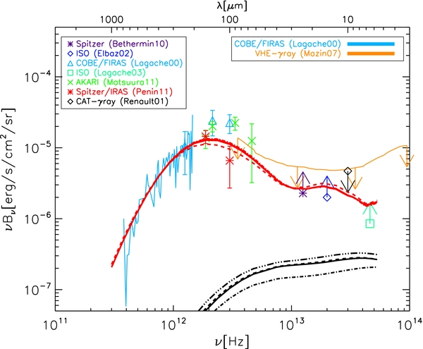
Figure 10. Cosmic IR background light. The red lines are model's predictions of the total radiation while black lines are just for the emission from SMBH dusty tori: solid line for reference variant, dashed line for fast_evol_SED_SF, dot-dashed line for low_IR2X_BH, and triple-dot-dashed line for high_IR2X_BH (see Table 1). All others are the observational constraints. References: Bethermin10: Béthermin et al. (2010); Elbaz02: Elbaz et al. (2002); Lagache00: Lagache & Puget (2000); Lagache03: Lagache et al. (2003); Matsuura11: Matsuura et al. (2011); Mazin07: Mazin & Raue (2007); Penin11: Pénin et al. (2012); Renault01: Renault et al. (2001).
Download figure:
Standard image High-resolution image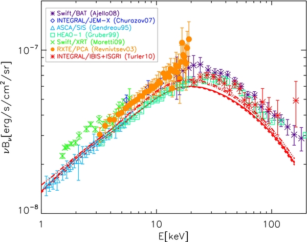
Figure 11. Cosmic X-ray background light. The red lines are the model's predictions: solid line for reference variant, dashed line for fast_evol_SED_SF, dot-dashed line for low_IR2X_BH, and triple-dot-dashed line for high_IR2X_BH (see Table 1). All others are the observational constraints. jello08: Ajello et al. (2008); Churazov07: Churazov et al. (2007); Gendreau95: Gendreau et al. (1995); Gruber99: Gruber et al. (1999); Moretti09: Moretti et al. (2009); Revnivtsev03: Revnivtsev et al. (2003); Turler10: Türler et al. (2010).
Download figure:
Standard image High-resolution image7.1. The SMBH Energy Fraction
As listed in Table 3 and shown in Figures 12 and 13, all variants of the model indicate that the median SMBH energy fraction in the total IR band increases with the IR luminosity, which is consistent with various studies in the local universe (e.g., Sanders & Mirabel 1996; Genzel et al. 1998; Armus et al. 2007; Desai et al. 2007; Veilleux et al. 2009; Petric et al. 2011) and at high-z (Kartaltepe et al. 2010), while the Gaussian width of the distribution increases with the decreasing luminosity. The overall trend of the median SMBH fraction with redshift shows a minimum around z ∼1–2. To test the robustness of this redshift trend, we first ran a model without redshift evolution (kBH1, d ≡ 0, kBH2, d ≡ 0) while all others are the same as those in the reference variant. The resulting best-fit reduced χ2 increased by as much as 1.3, which offers strong evidence for the requirement of redshift evolution in the SMBH energy fraction. We then ran a variant of the model that only allows monotonic evolution (i.e., kBH1, d = free, kBH2, d ≡ 0). The increase in the best-fit reduced χ2 is smaller but still significant by 0.4.

Figure 12. Median SMBH energy fraction in the total IR band as a function of the IR luminosity at four redshifts. The four variants of the model are shown with different line styles: solid line for reference variant, dashed line for fast_evol_SED_SF, dot-dashed line for low_IR2X_BH, and triple-dot-dashed line for high_IR2X_BH (see Table 1).
Download figure:
Standard image High-resolution image
Figure 13. Redshift evolution of the BH energy fraction at LTIR[L☉] = 12.3. Different line styles are for different variants of the model: solid line for reference variant, dashed line for fast_evol_SED_SF, dot-dashed line for low_IR2X_BH, and triple-dot-dashed line for high_IR2X_BH (see Table 1).
Download figure:
Standard image High-resolution imageIn Figure 14, we compared the 6.2 μm EWs in our model to several observed distributions at different redshifts, which offers a stringent check for our SMBH energy fraction measurements. Here the modeled samples are defined in similar ways to those observed. All EWs are measured using the spline interpolations, with the pure SF median value around 0.6–0.7 μm. Note that our SF templates do not have scatters in the EW, and thus the modeled EWs do not have values in bins higher than EW = 0.6–0.7 μm and any value below EW = 0.6 μm is caused by SMBH contributions in our model. At logLTIR = 12.3 and z = 0, the SMBH energy fraction in the model is fixed to that of 1 Jy ULIRGs, and is allowed to be luminosity and redshift-dependent. As shown in Figure 14(a) for ULIRGs, the model produces an almost flat trend, roughly consistent with the result of GOALS's ULIRGs (S. Stierwalt et al., in preparation) that additionally show excess objects in the lowest EW bin above a flat trend. For local LIRGs+ULIRGs, the distribution has a peak at the SF EW with a tail toward the low EW end, which is roughly consistent with the GOALS's result (S. Stierwalt et al., in preparation). Beyond the local universe, we compared the model's results to those of 5MUSES (Wu et al. 2010). At 0.05 < z < 0.3, the higher SF peak in the model compared to the observation is due to zero scatter in our SED templates. Overall, the SF peak plus a low EW tail as produced by the model is consistent with the observations. At 0.3 < z < 0.5, the model reproduces a bimodal EW distribution as observed, an SF peak plus a peak at the lowest bin with the latter higher than the former. For two higher redshift bins (0.5 < z < 1.0 and 1.0 < z < 2.0), the model reproduces a peak at the lowest bin with a tail toward the SF end as observed. In Figure 14, we also list the fraction of objects with EW < 0.4 for each observed or modeled distribution. This quantitative comparison further supports the consistency between the model's predictions and observations, with the former only slightly lower than the latter.
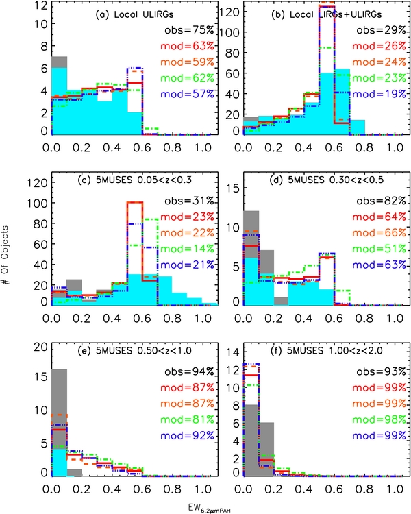
Figure 14. The 6.2 μm EW distributions. The cyan and gray filled histograms represent the observed detections and upper limits, respectively. The local LIRGs and ULIRGs are from S. Stierwalt et al. (in preparation), while those at higher redshifts are from 5MUSES (Wu et al. 2010). The open histograms are the model's predictions. Different line styles are for different variants of the model: solid line for the reference variant, dashed line for the fast_evol_SED_SF variant, dot-dashed line for the low_IR2X_BH variant, and triple-dot-dashed line for high_IR2X_BH (see Table 1). The listed percentages are the fractions of objects with EW < 0.4 for each distribution ("obs" stands for the observed distribution while "mod" is for the modeled distributions).
Download figure:
Standard image High-resolution image7.2. H i Column Density Distribution and Compton-thick AGN Fraction
The model characterizes the H i column density distribution through three bins, the type 1 (log cm2 < 22), Compton-thin type 2 (22 < log
 cm2 < 24), and Compton-thick AGNs (24 < log
 cm2 < 26). Figure 15 shows the evolution of the type 1 and Compton-thick AGN fractions in all AGNs as a function of the SMBH luminosity and redshift. All four variants of the model require that the type 1 fraction increases with the BH luminosity but decreases with redshift, and the CT fraction has the opposite trend.
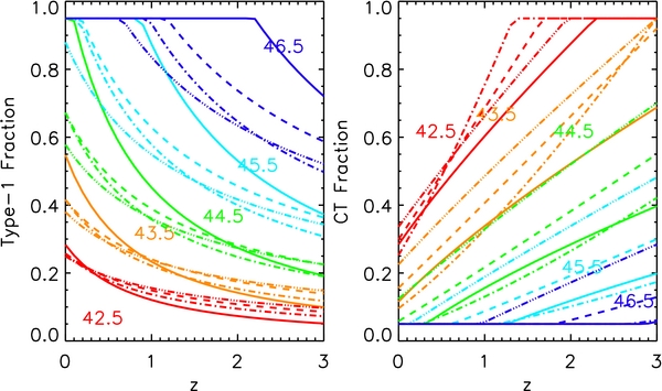
Figure 15. Redshift evolution of type 1 AGN fraction (left panel) and Compton-thick AGN fraction in all AGN populations. Different line styles are for different variants of the model: solid line for the reference variant, dashed line for the fast_evol_SED_SF variant, dot-dashed line for the low_IR2X_BH variant, and triple-dot-dashed line for high_IR2X_BH (see Table 1). Different colors are for different X-ray luminosities: blue for log(L2–10 keV(erg s−1)) = 42.5, cyan for log(L2–10 keV(erg s−1)) = 43.5, green for log(L2–10 keV(erg s−1)) = 44.5, orange for log(L2–10 keV(erg s−1)) = 45.5, red for log(L2–10 keV(erg s−1)) = 46.5.
Download figure:
Standard image High-resolution imageThe trend of the type 1 fraction with the SMBH luminosity is in general consistent with previous studies (e.g., Ueda et al. 2003; Hasinger 2004, 2008; La Franca et al. 2005; Barger et al. 2005; Treister et al. 2006; Ballantyne et al. 2006; Gilli et al. 2007). Although previous CXB models can explain the X-ray survey data either with the redshift dependence of the type 1 fraction (La Franca et al. 2005; Ballantyne et al. 2006) or without it (Ueda et al. 2003; Treister & Urry 2005; Gilli et al. 2007), the requirement of such a redshift evolution is highly preferred by our model, which is constructed to explain both the X-ray and IR data, consistent with recent studies of a large X-ray AGN sample (Hasinger 2008). Without redshift evolution (βz, type − 1 ≡ 0 & βz, CT ≡ 0), the best-fit reduced χ2 rises by 0.5, which is essentially caused by the increased brightness of high-z AGNs at both X-ray and 24 μm wavelengths. In the pure CXB model that only deals with the X-ray data, the increase in the apparent brightness of individual objects can be complemented by the decrease in the spatial number density in order to keep the number of objects above a given flux density unchanged. This is why the CXB model is not sensitive to redshift evolution of the type 1 fraction. However, the change of the AGN number density in our model is additionally constrained by the IR data. The redshift evolution of the break luminosity and density of the total IR LF is largely fixed throughout IR survey data. Although the change in the SMBH energy fraction can vary the AGN number densities, it also modifies the number density of the SF-dominated sources, especially the far-IR/submillimeter sources that lie at the bright end of the IR LF and thus are sensitive to the SMBH energy fraction. Without redshift evolution of the H i column density, the best-fit result shows that the redshift distributions at z > 1 of 24 μm sources brighter 5 mJy and 0.5–2 keV sources brighter than 10−14 erg s−1 cm−2 are overproduced by a factor of 10, and the redshift distribution of submillimeter sources systematically offsets by a factor of three along the Y-axis.
Our model requires a large number of the Compton-thick AGNs. At <10 keV, Compton-thick AGNs are extremely faint. The traditional CXB model first constrains the Compton-thin AGN through X-ray data at <10 keV and then add the Compton-thick AGN to match the CXB spectrum above 10 keV, especially the 20–30 keV peak (e.g., Ueda et al. 2003; Gilli et al. 2007). In this paper, we take advantage of the capability of the mid-IR data in probing these deeply buried AGNs thanks to significantly lower apparent gas-to-dust ratio. A test run of the model with zero Compton-thick AGN abundance shows that the reduced χ2 would worsen by as much as 1.0. The main reason is that the relative fraction between Compton-thick and Compton-thin type 2 AGNs as a function of the flux density is different at 24 μm from that at 0.5–2 and 2–10 keV, so that it is able to break the degeneracy between Compton-thick and Compton-thin type 2 AGNs seen in pure CXB models. As shown in Figure 16, the Compton-thick AGNs are only important over the faintest one to two orders of magnitude flux ranges in X-ray bands, while Compton-thin type 2 AGNs are important over a much larger flux ranges. The resulting Compton-thick to Compton-thin type 2 AGN fraction increases with the decreasing flux density at both bands. Such similar behaviors at both soft and hard bands imply that if the model is forced to replace Compton-thick objects with Compton-thin type 2 AGNs in one band, the result in the other band would not significantly violate the observation. However, at 24 μm, the Compton-thick contribution is noticeable over a flux range as large as four orders of magnitude, which is quite similar to that of the Compton-thin type 2 AGN. The relative ratio between the two populations is not a strong function of the flux density, with a value roughly around 1:3. This means that if the model is forced to replace Compton-thick AGNs with Compton-thin AGNs at 24 μm, the result in X-ray bands would significantly overproduce objects at the high flux end but underproduce them at the faint flux end. This argument was verified by running a test model without a Compton-thick AGN population and the expected behavior was observed in the model output.
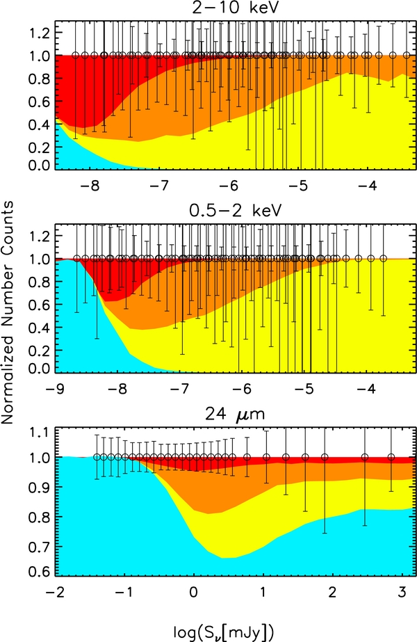
Figure 16. Percentage energy contributions to the number counts at 2–10 keV, 0.5–2 keV, and 24 μm, from different types of radiations in the reference model. Cyan for the pure star formation emission, yellow for the pure SMBH emission of type 1, orange for the pure SMBH emission of Compton-thin type 2, and red for the pure SMBH emission of Compton-thick AGNs.
Download figure:
Standard image High-resolution image7.3. The Total IR LF
As shown in Figure 17, the predicted total IR LFs are consistent with the observations over redshift and luminosity ranges where the data are available. For comparison, we converted the observed LFs at given filters to the total IR LFs using the reference variant. We first modeled the number density Φmodel(filter, z, νLν) at the same filter, redshift bin (z ± Δz), and luminosity bin (νLν ± ΔνLν) as the observed ones (Φobs(filter, z, νLν)). The νLν is then corrected to the total IR luminosity with luminosity corrections based on the probability-weighted average of all model SEDs within z ± Δz and νLν ± ΔνLν. This Φmodel/Φobs is taken as the difference of the observed and modeled LFs in the total IR band. For the local LFs, the IRAS data offer the largest dynamical range and are thus the best data set to test the validity of the model's LF. The 12 and 25 μm LFs are used to fit the model and the result is discussed in Section 6.3. Here we further compared our model to the total IR LF based on IRAS 60 μm selected sources (Sanders et al. 2003), and found a good match between the two (Figure 17). Consistency is excellent with other works of significantly smaller fields that cover the whole IR/submillimeter wavelength range. Above z > 0.1 up to z ∼ 3, current deep surveys are able to probe objects up to one order of magnitude below the break luminosity as shown in Figure 17. At short wavelengths (Wu et al. 2011; Rodighiero et al. 2010; Rujopakarn et al. 2010), no significant difference is found between the model and data up to z ∼ 2.5. Some deviations at the faint end are most likely caused by incompleteness corrections particularly associated with 1/Vmax method (Page & Carrera 2000). At rest-frame 250 μm, the model is consistent with that of Eales et al. (2010) but the result of Dye et al. (2010) is systematically higher at 0.1 < z < 0. The total IR LF of Caputi et al. (2007) is systematically above our modeled LF; their work may overestimate the total IR luminosity due to K-corrections (also see Magnelli et al. 2011).

Figure 17. Luminosity function in the total IR (8–1000 μm) at different redshifts. Different line styles are for different variants of the model: solid line for the reference variant, dashed line for the fast_evol_SED_SF variant, dot-dashed line for the low_IR2X_BH variant, and triple-dot-dashed line for high_IR2X_BH (see Table 1). References: Caputi07: Caputi et al. (2007); Dunne00: Dunne et al. (2000); Dye10: Dye et al. (2010); Eales10: Eales et al. (2010); Rodighiero10: Rodighiero et al. (2010); Rujopakarn10: Rujopakarn et al. (2010); Rush93: Rush et al. (1993); Sanders03: Sanders et al. (2003); Shupe98: Shupe et al. (1998); Vaccari10: Vaccari et al. (2010); Wu11: Wu et al. (2011).
Download figure:
Standard image High-resolution imageOur model hypothesizes no evolution in either the faint- or bright-end slopes of the total IR LF. As shown in Figure 17, the fixed bright-end slope matches the available data up to z ∼ 3. For the faint-end slope, we did not see deviations from the data up to z ∼ 1 above that which the available data are quite limited to justify. With fixed faint- and bright-end slopes, the total IR LF as predicted by our model requires evolution in both luminosity and density. Although the detail relies on the evolution formula adopted, we found in general that the break luminosity (logL*) increases with redshift but the break density (logΦ*) decreases with redshift. As shown in Figure 18, for the evolution formula given in Equations (2) and (3), the break luminosity increases rapidly until z = 2 and then gradually reaches the peak at z = 4, while the break density shows a gradual increase until z = 0.4 and then monotonically decreases with redshift. To test the redshift out to which luminosity or density evolution is required, we have carried out several test runs of the model by modifying the evolution formula to force no evolution above redshifts of z = 0.5, 1.0, 1.5, 2.0, 2.5, and 3.0. If we adopt Δχ2/dof = 1 as an indicator of significantly worse fit, we found that the no-evolution scenario can be ruled out below z ∼ 2.5. Above z ∼ 3, the fit result could not differentiate evolution versus no evolution, which is not surprising since the current constraint on the z > 3 infrared and X-ray populations is still of low statistical significance as, shown in Figure 7. To evaluate the degeneracy between the luminosity and density evolution, we carried out test runs that halted density or luminosity evolution at selected redshifts. The result shows that the data are not able to break the degeneracy at z ≳ 1.5, which is consistent with Figure 17 showing that above z ∼ 1.5 the observed LF does not extend significantly below the break luminosity. However, no matter which evolution formula is adopted, the robust result is that the break luminosity always increases with redshift, while the break density overall decreases with redshift. Our result of the positive luminosity evolution is consistent with different literature studies while the negative trend in the density is not always favored. We note that our result of negative density evolution is inconsistent with studies in Le Floc'h et al. (2005), Pérez-González et al. (2005), and Rodighiero et al. (2010), but consistent with ones in Caputi et al. (2007) and Magnelli et al. (2011).

Figure 18. Redshift evolution of four parameters describing the total IR LF including the break luminosity, break density, faint-end slope, and high-end slope. Different line styles are for different variants of the model: solid line for the reference variant, dashed line for the fast_evol_SED_SF variant, dot-dashed line for the low_IR2X_BH variant, and triple-dot-dashed line for high_IR2X_BH (see Table 1).
Download figure:
Standard image High-resolution image
8. CONCLUSIONS
In this paper, we have constructed a joint model of the X-ray and IR extragalactic background to account simultaneously for both the X-ray and IR survey data. The main conclusions are the following.
- 1.The model successfully fits the deep survey data with the scenario that individual galaxies are experiencing both SF and SMBH accretion activities. The model with 19 free parameters generates number counts, redshift distributions, and local LFs consistent with 617 data points over 6 decades of electromagnetic frequencies. The best-reduced χ2 reaches 2.7–2.9, with at least 0.75 contributed by cosmic variance, photo-z errors, or limitations of the data sets.
- 2.The unique output of this model, compared to previous ones for either pure X-ray or IR data, is to constrain the SMBH energy fraction in the total IR band. The best fit requires the SMBH energy fraction to increase with the IR luminosity but decrease with the redshift back to z ∼1.5. The derived trend is statistically significant as shown by the significantly increased best-fit χ2/dof, i.e., Δχ2/dof > 1.0, for best fits where the SMBH fraction has either no luminosity or no redshift dependence. An independent test comparing the model's predictions to the observed aromatic feature EW distributions agrees with this result.
- 3.The second important output of the model is the distribution of the H i column density obscuring the AGN, especially the Compton-thick fraction. A run of the model with a no-Compton-thick AGN shows an increase in the χ2/dof by ∼1.0. The best-fit parameters indicate that the Compton-thick AGN fraction decreases with the SMBH luminosity but increases with the redshift, while the type 1 AGN fraction has the inverse trend.
- 4.The third output is the total IR LF. The best-fit parameters indicate that the break luminosity rises monotonically with redshift while the break density has an overall inverse trend. The above result is statistically important out to z ∼ 1.5, above which the degeneracy between the two parameters cannot be resolved with available data.
We thank the anonymous referee for detailed and constructive comments. We thank Matthieu Bethermin for careful reading and comments. The work is supported through the Spitzer 5MUSES Legacy Program 40539. The authors acknowledge support by NASA through awards issued by JPL/Caltech.
Footnotes
- *
Online calculators of the model are available at http://5muses.ipac.caltech.edu/5muses/EBL_model/index.html.