


ABSTRACT
The next generation of space-based galaxy surveys is expected to measure the growth rate of structure to a level of about one percent over a range of redshifts. The rate of growth of structure as a function of redshift depends on the behavior of dark energy and so can be used to constrain parameters of dark energy models. In this work, we investigate how well these future data will be able to constrain the time dependence of the dark energy density. We consider parameterizations of the dark energy equation of state, such as XCDM and ωCDM, as well as a consistent physical model of time-evolving scalar field dark energy, ϕCDM. We show that if the standard, specially flat cosmological model is taken as a fiducial model of the universe, these near-future measurements of structure growth will be able to constrain the time dependence of scalar field dark energy density to a precision of about 10%, which is almost an order of magnitude better than what can be achieved from a compilation of currently available data sets.
Export citation and abstract BibTeX RIS
1. INTRODUCTION
Recent measurements of the apparent magnitude of Type Ia supernovae (SNeIa) continue to indicate, quite convincingly, that the cosmological expansion is currently accelerating (see, e.g., Conley et al. 2011; Suzuki et al. 2012; Li et al. 2011; Barreira & Avelino 2011).
If we assume that general relativity provides an adequate description of gravitational interactions on these cosmological length scales, then the kinematic properties of the universe can be derived by solving the Einstein equations
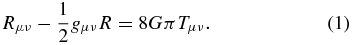
Here gμν is the metric tensor, Rμν and R are the Ricci tensor and (curvature) scalar respectively, Tμν is the stress-energy tensor of the universe's constituents, and G is the Newtonian gravitational constant.
There is good observational evidence that the large-scale radiation and matter distributions are statistically spatially isotropic. The (Copernican) cosmological principle, which is also consistent with current observations, then indicates that the Friedmann–Lemaître–Robertson–Walker (FLRW) models provide an adequate description of the spatially homogeneous background cosmological model.
In the FLRW models, the current accelerating cosmological expansion is a consequence of dark energy, the dominant, by far, term in the current cosmological energy budget. The dark energy density could be constant in time (and hence uniform in space)—Einstein's cosmological constant Λ (Peebles 1984)—or gradually decreasing in time and thus slowly varying in space (Peebles & Ratra 1988).
The "standard" model of cosmology is the spatially flat ΛCDM model in which the cosmological constant contributes around 75% of the current energy budget. Non-relativistic cold dark matter (CDM) is the next largest contributor, at around 20%, with non-relativistic baryons in third place with about 5%. For a review of the standard model, see Ratra & Vogeley (2008) and references therein.
Recent measurements of the anisotropies of the cosmic microwave background (CMB) radiation (e.g., Komatsu et al. 2011; Reichardt et al. 2012), in conjunction with significant observational support for a low density of non-relativistic matter (CDM and baryons together, e.g., Chen & Ratra 2003), as well as measurements of the position of the baryon acoustic oscillation (BAO) peak in the matter power spectrum (e.g., Percival et al. 2010; Dantas et al. 2011; Carnero et al. 2012; Anderson et al. 2012), provide significant observational support to the spatially flat ΛCDM model. Other data are also not inconsistent with the standard ΛCDM model. These include strong gravitational lensing measurements (e.g., Chae et al. 2004; Lee & Ng 2007; Biesiada et al. 2010), measurement of Hubble parameter as a function of redshift (e.g., Samushia & Ratra 2006; Sen & Scherrer 2008; Pan et al. 2010; Chen & Ratra 2011), large-scale structure data (e.g., Baldi & Pettrino 2011; De Boni et al. 2011; Brouzakis et al. 2011; Campanelli et al. 2011), and galaxy cluster gas mass fraction measurements (e.g., Allen et al. 2008; Samushia & Ratra 2008; Tong & Noh 2011). For recent reviews of the situation, see, e.g., Blanchard (2010), Sapone (2010), and Jimenez (2011).
While the predictions of the ΛCDM model are in reasonable accord with current observations, it is important to bear in mind that dark energy has not been directly detected (and neither has dark matter). Perhaps as a result of this, some feel that it is more reasonable to assume that the left-hand side of Einstein's equation (1) needs to be modified (instead of postulating a new, dark energy component of the stress-energy tensor on the right-hand side). While such modified gravity models are under active investigation, at present there is no compelling observational reason to prefer any of these over the standard ΛCDM cosmological model.
The ΛCDM model assumes that dark energy is a cosmological constant with equation of state

where  and
and  are the pressure and energy density of the cosmological constant (fluid). This minimalistic model, despite being in good agreement with most observations available today, has some potential conceptual shortcomings that have prompted research into alternative explanations of the dark energy phenomenon.3
To describe possible time dependence of the dark energy density, it has become popular to consider a more general equation-of-state parameterization

Here pω and ρω are the pressure and energy density of the dark energy fluid with redshift z dependent equation-of-state parameter ω(z). The simplest such parameterization is the XCDM one for which the equation-of-state parameter is constant and results in accelerated expansion if ω(z) = ωX < −1/3. In this case, the dark energy density decreases with time and this allows for the possibility that the fundamental energy density scale for dark energy is set at high energy in the early universe and the slow decrease of the energy density over the long age of the universe ensures that the characteristic dark energy density scale now is small (a few meV). This also ensures that the dark energy density remains comparable to the matter energy density over a longer period of time (compared to that for the ΛCDM model).
When ωX = −1, the XCDM parameterization reduces to the consistent (and complete) ΛCDM model. For any other value of ωX, the XCDM parameterization cannot consistently describe spatial inhomogeneities without further assumptions and extension (see, e.g., Ratra 1991; Podariu & Ratra 2000). Models in which ω(z) varies in time, ωCDM models, are also unable to consistently describe spatial inhomogeneities without further assumptions and extension.
A physically and observationally viable alternative to the ΛCDM model, which consistently describes a dark energy density slowly decreasing in time, is the ϕCDM model (Peebles & Ratra 1988; Ratra & Peebles 1988). This model, in which a dark energy scalar field, ϕ, slowly rolls down its potential, resulting in a slowly decreasing dark energy density, alleviates some of the conceptual problems, mentioned above, associated with the ΛCDM model. The slowly rolling scalar field, at a given instant of time, can be approximated by a dark energy fluid with an appropriately negative equation-of-state parameter.
More specifically, a ϕCDM model with an inverse-power-law scalar field potential energy density V(ϕ)∝ϕ−α, α > 0 is a prototypical example that has been extensively studied. This model has a nonlinear attractor or "tracker" scalar field solution that forces the initially sub-dominant dark energy density to come to dominate over the matter energy density, thus dominating the energy budget of the current universe, and so resulting in the current accelerated cosmological expansion. In addition to therefore partially alleviating the "coincidence" problem of the ΛCDM model, the ϕCDM model generates the current tiny dark energy scale of order an meV, measured by the SNeIa, through decrease, via cosmological expansion over the long age of the universe, of a much larger energy scale.
The α parameter controls the steepness of the scalar field potential, with larger values resulting in a stronger time dependence of the approximate equation-of-state parameter and α = 0 corresponds to the ΛCDM model limit. α has been constrained using currently available data (see, e.g., Chen & Ratra 2004, 2012; Wilson et al. 2006; Mania & Ratra 2012, and references therein). The strongest current limits are that α has to be less than ∼0.7 at 2σ confidence (Samushia 2009).
In the ϕCDM model, or in the XCDM or ωCDM parameterizations, the background evolution of the (spatially homogeneous) universe differs from that in the ΛCDM case. This affects both the distance–redshift relation as well as the growth rate of large-scale structure. With precise measurements of distance and growth rate over a range of redshifts it will be possible to discriminate between cosmological models.4
The BAO signature in the observed large-scale structure of the universe allows for the measurements of radial and angular distances as functions of redshift (see, e.g., Percival et al. 2010; Blake et al. 2011b; Beutler et al. 2011; Anderson et al. 2012). In addition, the redshift-space distortion signal allows for inferences about the strength of gravitational interactions on very large scales (see, e.g., Percival & Schäfer 2004; Angulo et al. 2007; Guzzo et al. 2008; Blake et al. 2011a; Samushia et al. 2012; Reid et al. 2012). Currently available data sets have been used to measure distances and growth history up to a redshift z ∼ 0.8 and the next generation of planned space-based galaxy redshift surveys of the whole extragalactic sky is expected to extend these measurements to a redshift z ∼ 2. Possible candidates for such surveys include the Euclid satellite mission that has been approved by the European Space Agency (Laureijs et al. 2011) and the WFIRST satellite that was ranked high by the recent Decadal Survey (Green et al. 2011). These surveys have been shown to have the potential to measure angular distances, Hubble parameter H(z), and growth rate as functions of redshift to precision of a few percent over a wide range of redshifts (Wang et al. 2010; Samushia et al. 2011; Majerotto et al. 2012; Basse et al. 2012).5
As mentioned above, an alternative potential explanation of the observed accelerated expansion of the universe is to replace general relativity by a modified theory of gravity. For example, in the f(R)-gravity models the Einstein–Hilbert gravitational action is modified to
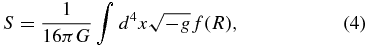
where the function f(R) of the Ricci curvature R can in general be of any form. In the special case when f(R) = R, one recovers the Einstein–Hilbert action which yields the Einstein equations of general relativity, Equation (1). For every dark energy model it is possible to find a function f(R) that will result in exactly the same expansion history (see, e.g., Sotiriou & Faraoni 2010; Tsujikawa 2010; Capazziello & De Laurentis 2011), thus potentially eliminating the need for dark energy. However, nothing prevents the coexistence of modified gravity and dark energy, with both contributing to powering the current accelerated cosmological expansion. It is of significant importance to be able to determine which scenario best describes what is taking place in our universe.
In this paper, we investigate how well anticipated data from the galaxy surveys mentioned above can constrain the time dependence of the dark energy. We will use the Fisher matrix formalism to obtain predictions for the ϕCDM model and compare these with those made using the (model-dependent) XCDM and ωCDM parameterizations of dark energy. We will mostly assume that gravity is well described by general relativity, but will also look at some simple modified gravity cases. We find that the anticipated constraints on the parameter α of the ϕCDM model are almost an order of magnitude better than the ones that are currently available.
Compared to the recent analysis of Samushia et al. (2011), here we use an updated characterization of planned next-generation space-based galaxy surveys, so our forecasts are a little more realistic. We also consider an additional dark energy parameterization, XCDM, a special case of ωCDM that was considered by Samushia et al. (2011), as well as the ϕCDM model, forecasting for which has not previously been done.
The paper is organized as follows. In Section 2, we briefly describe the observables and their relationship to basic cosmological parameters. In Section 3, we describe the models of dark energy that we study. Section 4 outlines the method we use for predicting parameter constraints, with some details given in the Appendix. We present our results in Section 5 and conclude in Section 6.
2. MEASURED POWER SPECTRUM OF GALAXIES
The large-scale structure of the universe, which most likely originated as quantum-mechanical fluctuations of the scalar field that drove an early epoch of inflation (see, e.g., Fischler et al. 1985), became (electromagnetically) observable at z ∼ 103 after the recombination epoch. Dark energy did not play a significant role at this early recombination epoch because of its low mass-density relative to the densities of ordinary and dark matter as well as that of radiation (neutrinos and photons). At z ∼ 5, galaxy clusters began to form. Initially, in regions where the matter density was a bit higher than the average, space expanded a bit slower than average. Eventually, the dark and ordinary matter reached a minimum density and the regions contracted. If an overdense region was sufficiently large, its baryonic matter collapsed into its dark-matter halo. The baryonic matter continued to contract even more due to its ability to lose thermal energy through the emission of electromagnetic radiation. This cannot happen with dark matter since it does not emit significant electromagnetic radiation nor does it interact significantly (non-gravitationally) with baryonic matter. As a result the dark matter remained in the form of a spherical halo around the rest of the baryonic part of a galaxy. At z ∼ 2, the rich clusters of galaxies were formed by gravity, which gathered nearby galaxies together. Also, by this time the dark energy's energy density had become relatively large enough to affect the growth of large-scale structure.
Different cosmological models with different sets of parameters can result in the same expansion history and so it is impossible to distinguish between such models by using only expansion history measurements. This is one place where measurements of the growth history of the large-scale structure of the universe play an important role. It is not possible to fix free parameters of two different cosmological models to give exactly the same expansion and growth histories simultaneously. It is therefore vital to observe both histories in order to obtain better constraints on parameters of a cosmological model.
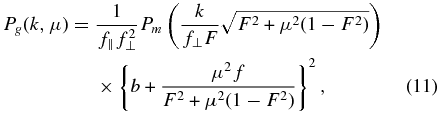
In a cosmological model described by the FLRW metric, and to lowest order in dark matter overdensity perturbations, the power spectrum of observed galaxies is given by (Kaiser 1987)

Here subscript g denotes galaxies, Pm is the underlying matter power spectrum, b is the bias of galaxies, f is the growth rate, μ is the cosine of the angle between wavevector k and the line-of-sight direction, and σ8 is the overall normalization of the power spectrum (σ8 is the rms energy density perturbation smoothed over spheres of radius 8 h−1 Mpc, where h = H0/(100 km s−1 Mpc−1) and H0 is the Hubble constant). Since, for a measured power spectrum of galaxies on a single redshift slice, the bias and growth rate are perfectly degenerate with the overall amplitude, in the equations below we will refer to bσ8 and fσ8 simply as b and f.
The angular dependence of the power spectrum in Equation (5) can be used to infer the growth rate factor f(z) which is defined as the logarithmic derivative of the linear growth factor
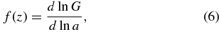
where a is the cosmological scale factor, and the linear growth factor G(t) = δ(t)/δ(tin) shows by how much the perturbations have grown since some initial time tin.6
The numerical value of the f(z) function depends both on the theory of gravity and on the expansion rate of the universe. Since the growth rate depends very sensitively on the total amount of non-relativistic matter, it is often parameterized as (see, e.g., Linder 2005, and references therein)

where
and

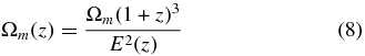
Here H(z) is the Hubble parameter and H0 is its value at the present epoch (the Hubble constant), Ωm is the value of the energy density parameter of non-relativistic matter at the present epoch (z = 0), Ωk that of spatial curvature, and ΩDE(z) is the energy density parameter which describes the evolution of the dark energy density and is different in different dark energy models.
The growth index, γ, depends on both a model of dark energy as well as a theory of gravity. When general relativity is assumed and the equation of state of dark energy is taken to be of the general form in Equation (3), then (see, e.g., Linder 2005, and references therein)

to a few percent accuracy. In the ΛCDM cosmological model γ ≈ 0.55. An observed significant deviation from this value of γ will present a serious challenge for the standard cosmological model.
The power spectrum is measured under the assumption of a fiducial cosmological model. If the angular and radial distances in the fiducial model differ from those in the real cosmology, the power spectrum will acquire an additional angular dependence via the Alcock & Paczyński (1979, AP) effect, as discussed in Samushia et al. (2011),
where


Here Rr = dr/dz is the derivative of the radial distance, DA is the angular diameter distance (both defined below), a hat indicates a quantity evaluated in the fiducial cosmological model, and a quantity without a hat is evaluated using the alternative cosmological model. The AP effect is an additional source of anisotropy in the measured power spectrum and allows for the derivation of stronger constraints on cosmological parameters.
3. COSMOLOGICAL MODELS
In an FLRW model with only non-relativistic matter and dark energy the distances DA(z) and Rr(z) are
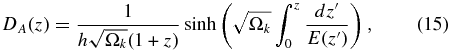
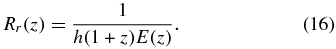
Here E(z) is defined in Equation (9). The functional form of E(z) depends on the model of dark energy.
3.1. ΛCDM, XCDM, and ωCDM Parameterizations
Here we describe the relevant features of the ΛCDM model and the dark energy parameterizations we consider.
If the dark energy is taken to be a fluid, its equation of state can be written as p = ω(z)ρ. For the ΛCDM model the equation-of-state parameter ω(z) = −1 and the dark energy density is time independent.
In the XCDM parameterization ω(z) = ωX(< − 1/3) is allowed to take any time-independent value, resulting in a time-dependent dark energy density.
In the ωCDM parameterization the time dependence of ω(z) is parameterized by introducing an additional parameter ωa through (Chevallier & Polarski 2001; Linder 2003)
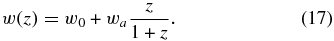
The XCDM parameterization is the limit of the ωCDM parameterization with ωa = 0. In the ωCDM parameterization the function ΩDE(z) that describes the time evolution of the dark energy density is
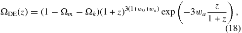
and the corresponding expression for the XCDM case can be derived by setting ωa = 0 here.
3.2. ϕCDM Model
In the ϕCDM model the energy density of the background, spatially homogeneous, scalar field ϕ can be found by solving the set of simultaneous ordinary differential equations of motion,
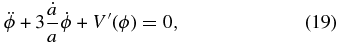
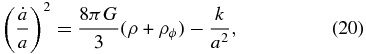
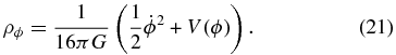
Here an overdot denotes a derivative with respect to time, a prime denotes one with respect to ϕ, V(ϕ) is the potential energy density of the scalar field, ρϕ is the energy density of the scalar field, and ρ is the energy density of the other constituents of the universe.
Following Peebles & Ratra (1988) we consider a scalar field with inverse-power-law potential energy density
Here α is a positive parameter of the model to be determined experimentally and κ is a positive constant. This choice of potential has the interesting property that the scalar field solution is an attractor with an energy density that slowly comes to dominate over the energy density of the non-relativistic matter (in the matter-dominated epoch) and causes the cosmological expansion to accelerate. The function ΩDE(z) in the case of ϕCDM is
4. FISHER MATRIX FORMALISM
The precision of the galaxy power spectrum measured in redshift bins depends on the cosmological model, the volume of the survey, and the distribution of galaxies within the observed volume. See the Appendix for a summary of how to estimate the precision of measurements from survey parameters.
We assume that the power spectrum P(ki)meas has been measured in N wavenumber ki bins (i = 1...N) and each measurement has a Gaussian uncertainty σi. From these measurements a likelihood function
can be constructed, where
Here  are the set of cosmological parameters on which the power spectrum depends.
The likelihood function in Equation (24) can be transformed into the likelihood of theoretical parameters  by Taylor expanding it around the maximum and keeping terms of only second order in
  as χ2(δp) = Fjkδpjδpk, where Fjk is the Fisher matrix7 of the parameter set
  given by second derivatives of the likelihood function through
The Fisher matrix predictions are exact in the limit where initial measurements as well as derived parameters are realizations of a Gaussian random variable. This would be the case if the Pmeasi were perfectly Gaussian and the  were linear functions of
  , which would make the second-order Taylor expansion of the likelihood around its best-fit value exact. In reality, because of initial non-Gaussian contributions and nonlinear effects, the predictions of Fisher matrix analysis will be different (more optimistic) from what is achievable in practice. These differences are larger for strongly nonlinear models and for the phase spaces in which the likelihood is non-negligible at some physical boundary (α = 0 in the case of ϕCDM). A more realistic approach that requires significantly more computational time and power is to generate a large amount of mock data and perform a full Monte Carlo Markov Chain (MCMC) analysis (see, e.g., Perotto et al. 2006; Martinelli et al. 2011, where the authors find significant differences compared to the results of the Fisher matrix analysis).
We assume that the full-sky space-based survey will observe Hα-emitter galaxies over 15,000 deg2 of the sky. For the density and bias of observed galaxies we use predictions from Orsi et al. (2010) and Geach et al. (2010), respectively. We further assume that about half of the galaxies will be detected with a reliable redshift. These numbers roughly mirror what proposed space missions, such as the ESA Euclid satellite and the NASA WFIRST mission, are anticipated to achieve. For the fiducial cosmology we use a spatially flat ΛCDM model with Ωm = 0.25, the baryonic matter density parameter Ωb = 0.05, σ8 = 0.8, and the primordial density perturbation power spectral index ns = 1.0; for convenience we summarize all the parameters of the fiducial model in Table 1.
Table 1. Values of the Parameters of the Fiducial ΛCDM Model and the Survey
| Ωm | Ωb | Ωk | h | σ8 | ns | Efficiency | Redshift Span | Covered Sky Area |
|---|---|---|---|---|---|---|---|---|
| (deg2) | ||||||||
| 0.25 | 0.05 | 0.0 | 0.7 | 0.8 | 1.0 | 0.45 | 0.55 ⩽z ⩽ 2.05 | 15000 |
Download table as: ASCIITypeset image
We further assume that the shape of the power spectrum is known perfectly (for example, from the results of the Planck satellite) and ignore derivatives of the real-space power spectrum with respect to cosmological parameters.
We predict the precision of the measured galaxy power spectrum and then transform it into correlated error bars on the derived cosmological parameters. At first, we make predictions for the basic quantities b and f in the XCDM and ωCDM parameterizations and in the ϕCDM model. Then it allows us to predict constraints on deviations from general relativity and see how these results change with changing assumptions about dark energy. Finally, we forecast constraints on the basic cosmological parameters of dark energy models.
For the XCDM parameterization, these basic cosmological parameters are pXCDM = (f, b, h, Ωm, Ωk, wX). The ωCDM parameterization has one extra parameter describing the time evolution of the dark energy equation-of-state parameter, pωCDM = (f, b, h, Ωm, Ωk, w0, wa). For the ϕCDM model, the time dependence of the dark energy density depends only on one parameter α so we have pϕCDM = (f, b, h, Ωm, Ωk, α). In order to derive constraints on the parameters of the considered cosmological models while altering assumptions about the correctness of general relativity, we transform Fisher matrices of each model from the parameter set described above to the following parameter set (that now includes γ that parameterizes the growth rate) pmodel = (γ, model), where by model we mean all the parameters of a particular model, for example, for ωCDM model = pωCDM = (f, b, h, Ωm, Ωk, w0, wa).
5. RESULTS
5.1. Constraints on Growth Rate
Figure 1 shows predictions for the measurement of growth rate assuming different dark energy models. We find that in the most general case, when no assumption is made about the nature of dark energy, the growth rate can be constrained to a precision of better than 2% over a wide range of redshifts. This is in good agreement with previous similar studies (see, e.g., Figure 1 of Samushia et al. 2011). When we specify a dark energy model, the constraints on growth rate improve by about a factor of two. There is very little difference between the results derived for different dark energy models: the precision is almost insensitive to the assumed model. Also, one can note that the curves for the XCDM parameterization and for the ϕCDM model are almost identical. The likely explanation of this effect is that for a fixed redshift bin the ϕCDM model is well described by the XCDM parameterization with the value of the parameter ωX = pϕ/ρϕ, where the values of the scalar field pressure pϕ and energy density ρϕ are evaluated at that redshift bin.
Figure 1. Predicted relative error on the measurements of growth rate as a function of redshift z in redshift bins of Δz = 0.1 for different models of dark energy. The upper solid black line shows predictions for the case when no assumption is made about the nature of dark energy.
Download figure:
Standard image High-resolution imageThe measurements of growth rate can be remapped into constraints on parameters describing the deviation from general relativity. Figure 2 shows correlated constraints between the current renormalized Hubble constant h and the γ parameter that describes the growth of structure. The ϕCDM model constraints on both h and γ are tighter than those for the XCDM or ωCDM parameterizations. As expected, the most restrictive ΛCDM model results in the tightest constraints. In Table 2, we show how the constraint on the γ parameter depends on the adopted dark energy model.
Figure 2. Predicted one standard deviation confidence level contour constraints on the current renormalized Hubble constant h and the parameter γ that describes deviations from general relativity for different dark energy models.
Download figure:
Standard image High-resolution imageTable 2. Predicted Deviations of Parameter γ from its Fiducial Value, at One Standard Deviation Confidence Level, for Different Assumptions about Dark Energy
| DE Model | Fiducial γ | Deviation |
|---|---|---|
| ωCDM | 0.55 | 0.035 |
| ϕCDM | 0.55 | 0.023 |
| XCDM | 0.55 | 0.035 |
| ΛCDM | 0.55 | 0.016 |
Download table as: ASCIITypeset image
5.2. Constraints on Dark Energy Model Parameters
We use measurements of growth and distance to constrain parameters of the dark energy models.
Figure 3 shows constraints on parameters of the ωCDM parameterization (these should be compared to Figures 4(a) and 5(a) of Samushia et al. 2011). When no assumptions are made about the nature of gravity, the constraints on ω0 and ωa are very weak and degenerate. When we assume general relativity, the constraints tighten significantly, resulting in ∼10% accuracy in the measurement of ω0 and ∼25% accuracy in the measurement of ωa.
Figure 3. Upper panel shows one standard deviation confidence level contour constraints on parameters ωa and ω0 of the ωCDM parameterization, while lower panel shows these for parameters Ωk and Ωm.
Download figure:
Standard image High-resolution imageThe upper panel of Figure 4 shows constraints on the parameters ωX and Ωm of the XCDM parameterization. Similar to the previous case, the constraints tighten significantly when we assume general relativity as the model of gravity. About a 2% measurement of ωX and a 5% measurement of Ωm are possible in this case. The lower panel of Figure 4 shows the related constraints on Ωk and Ωm for the XCDM parameterization. The constraints are similar to, but somewhat tighter than, those for the ωCDM parameterization. This is because the XCDM parameterization has one less parameter than the ωCDM parameterization. Spatial curvature can be constrained to about 15% precision in this case.
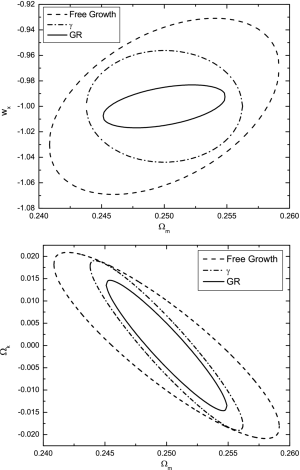
Figure 4. One standard deviation confidence level contour constraints on parameters of the XCDM parameterization.
Download figure:
Standard image High-resolution imageFigures 5 and 6 show constraints on parameters of the ϕCDM model. In the most general case, when no assumption is made about the nature of gravity, the constraints are weak and the parameters α and Ωm are strongly correlated, with larger values of α requiring larger values of Ωm. When general relativity is assumed, the constraints become much stronger and parameter α can be constrained to be less than 0.1 at the 1σ confidence level. This is significantly better than any constraint available at the moment.
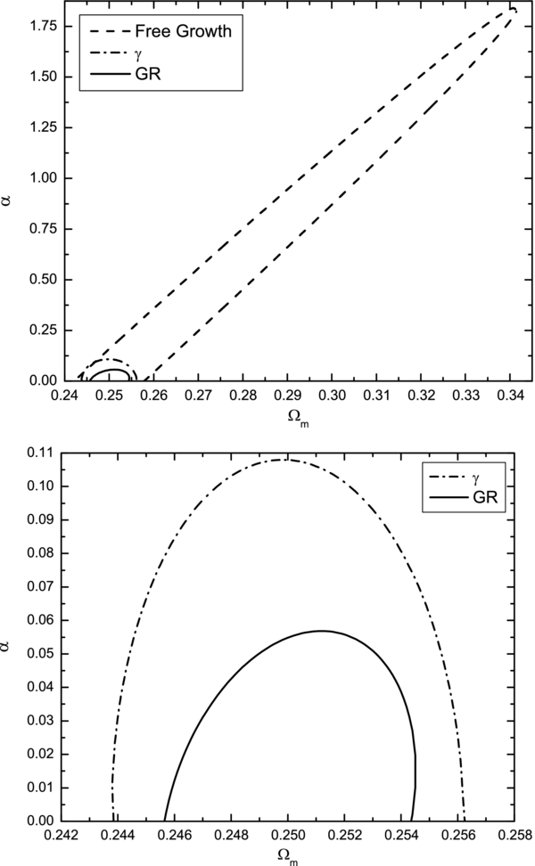
Figure 5. One standard deviation confidence level contour constraints on parameters α and Ωm of the ϕCDM model. Lower panel shows a magnification of the tightest two contours in the lower left corner of the upper panel.
Download figure:
Standard image High-resolution image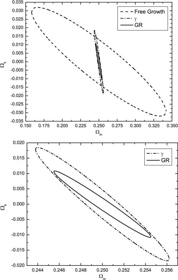
Figure 6. One standard deviation confidence level contour constraints on parameters Ωk and Ωm of the ϕCDM model. The lower panel shows a magnification of the two tightest contours in the center of the upper panel.
Download figure:
Standard image High-resolution imageFigure 7 shows constraints on the parameters of the ΛCDM model. From the clustering data alone, the spatial curvature can be constrained with almost 1% precision, largely because this model has the least number of free parameters.
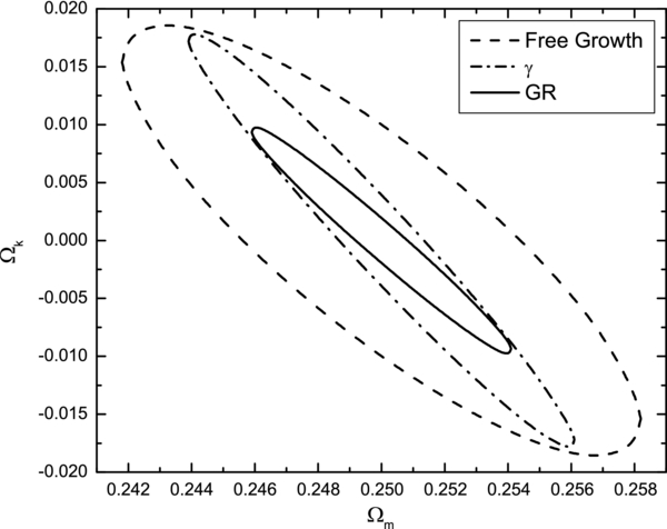
Figure 7. One standard deviation confidence level contour constraints on parameters Ωk and Ωm of the ΛCDM model.
Download figure:
Standard image High-resolution imageThe exact numerical values for the forecast error bars and likelihood contours should be taken with caution and not be interpreted as predictions for the performance of any specific survey (such as Euclid or WFIRST). Our main objective in this work was first to investigate how the modified gravity constraints change with different models of dark energy and second to demonstrate the improvement in ϕCDM model constraints achievable with future galaxy surveys. Because of this we were able to simplify our method by adopting a Fisher matrix formalism instead of a full MCMC approach and also use a simplified description of the survey baseline. For more realistic predictions of Euclid performance, see, e.g., Laureijs et al. (2011), Samushia et al. (2011), and Majerotto et al. (2012).
6. CONCLUSION
We have forecast the precision at which planned near-future space-based spectroscopic galaxy surveys should be able to constrain the time dependence of dark energy density. For the first time, we have used a consistent physical model of time-evolving dark energy, ϕCDM, in which a minimally coupled scalar field slowly rolls down its self-interaction potential energy density. We have shown that if general relativity is assumed, the deviation of the parameter α of the ϕCDM model can be constrained to better than 0.05; this is almost an order of magnitude better than the best currently available result.
The constraints on basic cosmological parameters, such as the relative energy densities of non-relativistic matter and spatial curvature, depend on the adopted dark energy model. We have shown that in the ϕCDM model the expected constraints are more restrictive than those derived using the XCDM or ωCDM parameterizations. This is due to the fact that the ϕCDM model has fewer parameters. Also, the XCDM and ωCDM parameterizations assign equal weight to all possible values of ω, while in the ϕCDM model there is an implicit theoretical prior on which equation-of-state parameter values are more likely, based on how easy it is to produce such a value within the model.
Since the observational consequences of dark energy and modified gravity are partially degenerate, constraints on modified gravity parameters will depend on the assumptions made about dark energy. The constraints on γ are most restrictive in the ΛCDM model. For the ϕCDM model, the constraints on γ are about a third tighter than those for the ωCDM and XCDM parameterizations.
These results are very encouraging: data from an experiment of the type we have modeled will be able to provide very good, and probably revolutionary, constraints on the time evolution of dark energy.
This work was supported by DOE grant DEFG030-99EP41093 and NSF grant AST-1109275. L.S. is grateful for support from European Research Council, SNSF SCOPES grant # 128040, and GNSF grant ST08/4-442.
APPENDIX
In this Appendix, we summarize how to estimate the precision of measurements from the survey parameters.
The Fisher matrix coefficients are given by
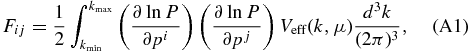
where the effective volume is
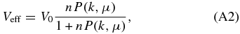
and V0 is the total survey volume and n is the number density. Also, following Tegmark (1997), we multiply the integrand in Equation (A1) by a Gaussian factor exp (− k2σz(dr(z)/dz)), where r(z) is the comoving distance, in order to account for the errors in distance induced by the errors of redshift measurements, σz = 0.001. We model the theoretical power spectrum using an analytic approximation of Eisenstein & Hu (1998). We integrate in k from kmin = 0 to kmax, where the kmax values depend on redshift and are chosen in such a way that the small scales that are dominated by nonlinear effects are excluded. The range of scales that will be fitted to the future surveys will depend on how well the theoretical templates are able to describe small-scale clustering and is difficult to predict. The kmax values along with the expected bias and number density of galaxies are listed in Table 3.
Table 3. Values of the kmax, Bias b(z) from Orsi et al. (2010), and the Number Densities n(z) Taken from Geach et al. (2010)
| z | kmax | b(z) | n(z) |
|---|---|---|---|
| 0.55 | 0.144 | 1.0423 | 3220 |
| 0.65 | 0.153 | 1.0668 | 3821 |
| 0.75 | 0.163 | 1.1084 | 4364 |
| 0.85 | 0.174 | 1.1145 | 4835 |
| 0.95 | 0.185 | 1.1107 | 5255 |
| 1.05 | 0.197 | 1.1652 | 5631 |
| 1.15 | 0.2 | 1.2262 | 5972 |
| 1.25 | 0.2 | 1.2769 | 6290 |
| 1.35 | 0.2 | 1.2960 | 6054 |
| 1.45 | 0.2 | 1.3159 | 4985 |
| 1.55 | 0.2 | 1.4416 | 4119 |
| 1.65 | 0.2 | 1.4915 | 3343 |
| 1.75 | 0.2 | 1.4873 | 2666 |
| 1.85 | 0.2 | 1.5332 | 2090 |
| 1.95 | 0.2 | 1.5705 | 1613 |
| 2.05 | 0.2 | 1.6277 | 1224 |
Download table as: ASCIITypeset image
In order to derive the Fisher matrix of a specific cosmological model, we have to go from our initial parameter space to the parameter space of the cosmological model whose Fisher matrix we want. The transformation formula for the Fisher matrix is given by (see, e.g., Albrecht et al. 2009, for a review)
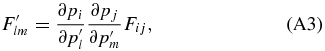
where the primes denote the "new" Fisher matrix and parameters.
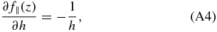
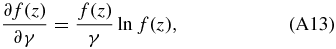
We now list the derivatives of the transformation coefficients of the ϕCDM model in the limit  0 and
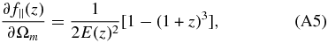
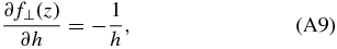
0 and  0 (which corresponds to the fiducial spatially flat ΛCDM model). The transformation coefficients relating f∥(z) and the parameters (h, Ωm, Ωk, α) are
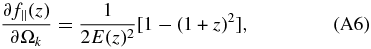
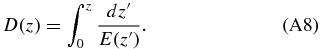
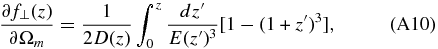
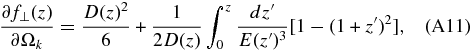
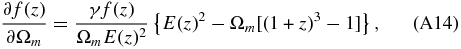
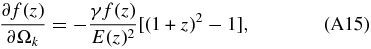
For the other transformation coefficients, it is convenient to introduce the integral
Then the transformation coefficients between f⊥(z) and the parameters (h, Ωm, Ωk, α) are
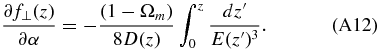
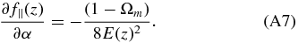
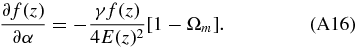
Finally, the transformation coefficients between the growth factor f(z) and the parameters (γ, h, Ωm, Ωk, α) are
Footnotes
- 3
- 4
There are many other models under current discussion, besides the ΛCDM and ϕCDM models and XCDM and ωCDM parameterizations we consider here for illustrative purposes. For a sample of the available options see, e.g., Yang et al. (2011); Frolov & Guo (2011); Nunes et al. (2011); Grande et al. (2011); Saitou & Nojiri (2011); Silva et al. (2010); Kamenshchik et al. (2011); Maggiore et al. (2011).
- 5
For constraints on cosmological parameters from data from space missions proposed earlier, see Podariu et al. (2001) and references therein.
- 6
Here we have expanded the energy density
 in terms of a small spatially inhomogeneous fractional perturbation about a spatially homogeneous background ρb(t): .
 - 7
For a review of the Fisher matrix formalism as applied to cosmological forecasting, see Albrecht et al. (2009).


![$\rho (t,{{\bm x}}) = \rho _b(t) [ 1 + \delta (t, {{\bm x}})]$](https://content.cld.iop.org/journals/0004-637X/760/1/19/revision1/apj447606ieqn5.gif)