


ABSTRACT
Non-redundant aperture masking interferometry with adaptive optics (AO) is a powerful technique for high contrast at the diffraction limit with high-precision astrometry and photometry. A limitation to the achievable contrast can be attributed to spatial fluctuations of the wavefront—those within a sub-aperture and across sub-apertures—and temporal fluctuations within a single exposure. Spatial filtering addresses spatial fluctuations within a sub-aperture. An optimized pinhole in the focal place preceding the aperture mask is one approach for reducing the variation of the wavefront within a sub-aperture. Similarly, a weak spatial filtering effect is shown to be provided by post-processing the images with an apodized window function, typically used to minimize detector read noise and contamination from wide-separated sources. We explore the effects of spatial filtering through calculation, simulation, and observational tests conducted with a pinhole and aperture mask in the PHARO instrument at the Hale 200'' Telescope at Palomar Observatory. We find that a pinhole decreases stochastic closure phase errors and calibration errors, but that tight restrictions are placed onto the alignment of binary targets within the pinhole. We propose an observation strategy to relax these restrictions. If implemented, the pinhole could potentially yield an increase in achievable contrast by up to 10%–25% in H and Ks bands, and more at very high Strehl (≳80%). We also conclude that correcting low-order wavefront modes within the sub-apertures will be key for reaching high contrasts with extreme-AO systems such as the Gemini Planet Imager and PALM3K to search for planets.
Export citation and abstract BibTeX RIS
1. INTRODUCTION
Current planetary searches using a coronagraph (e.g., Hinkley et al. 2011) excel at obtaining very high contrast (105:1) but are unable to probe at close separations (≲300–500 mas) where the field of view is blocked by the occulting spot. This separation rules out the observation at physical separations ≲10 AU for many host stars. The detection of planetary companions with techniques providing both high contrast and high resolution will play a key role in identifying the full distribution of Jupiter-class planets and for investigating the mechanisms of planetary formation (Kraus et al. 2009), migration, and stability (Veras et al. 2009; Raymond et al. 2009 and, e.g., HR 8799, Fabrycky & Murray-Clay 2010).
Non-Redundant Aperture Masking Interferometry (NRM or aperture masking) in conjunction with adaptive optics (AO) is well established for yielding much more precise astrometry and photometry than AO alone at close separations (e.g., Kraus et al. 2008, 2011) and for the detection of high-contrast companions (Lloyd et al. 2006). The application of aperture masking with AO on 5–10 m class telescopes achieves contrasts of 102–103:1 at and outward of λ/D and nicely complements companion searches with a coronagraph. The increased contrast and resolution of NRM has been used with great effect for stellar multiplicity studies (Kraus et al. 2008, 2011), the detection of short-period brown dwarfs for dynamical mass measurements (Lloyd et al. 2006; Bernat et al. 2010), and a high-contrast search for inner planetary companions to HR 8799 (Hinkley et al. 2011). With the Gemini Planet Imager (Macintosh et al. 2008) and Project 1640 IFS (Hinkley et al. 2009) equipped with non-redundant masks, aperture masking interferometry from the ground will play a key role in the detection of exoplanets at close separations.
NRM observations use a mask to transform the full telescope aperture into a sparsely populated set of sub-apertures, constructed so that no two pairs of sub-apertures share the same baseline direction and length (i.e., are non-redundant). The strength of this technique draws on its measurement of the closure phase quantity (e.g., Jennison 1958; Readhead et al. 1988; Cornwell 1989), an observable that naturally mitigates the effect of wavefront errors on scales larger than a sub-aperture. These same wavefront errors produce the speckles of direct imaging, which dominate the image noise by orders of magnitude whether arising from atmospheric variation (Racine et al. 1999) or quasi-static instrumental effects (Hinkley et al. 2007). Their mitigation by closure phases enables higher contrast despite the blocking of 90%–95% of the flux by the aperture mask.
The achievable contrast of the technique is limited by its own calibration challenges, one of which arises from quasi-static spatial variation of the wavefront within the sub-aperture. Such wavefront errors erode the effectiveness of using closure phases (resulting in redundancy noise in the language of Readhead et al. 1988 and others). Similarly, decreasing the wavefront variation within the sub-aperture can increase the contrast of NRM observations further.
Optical and infrared long-baseline interferometers have implemented single-mode fibers and pinholes which spatially filter (i.e., smooth) aperture wavefront errors to improve measurements of complex visibility (Shaklan & Roddier 1987; du Foresto et al. 1997). Poyneer & Macintosh (2004) have studied the use of a pinhole to develop an AO wavefront sensor which more accurately measures the wavefront above a sub-aperture. Likewise, spatially filtering the wavefront errors with a pinhole placed in the image (focal) plane before the aperture mask may provide a means for substantially increasing the achievable contrast of NRM observations.
This paper provides a comprehensive analysis of NRM with pinhole spatial filtering. To establish its theoretical foundation, we present an analytic description of the combined technique (Section 2). Using an accurate simulation of an aperture masking equipped telescope, we derive the optimal pinhole size and estimate its expected performance, limitations, and restrictions. We also derive several results applicable to general aperture masking observations. (Sections 3 and 4). We have also installed a pinhole in the PHARO instrument of the Hale 200'' Telescope at Palomar Observatory. To study how spatial filtering improves the sensitivity of NRM observations and influences the astrometric and photometric characterization of discovered binary systems, we observed 26 single stars and 4 known binaries with and without the pinhole (Section 5). This paper further develops the understanding of NRM as a technique for detecting high-contrast companions and provides several new findings to guide the design of NRM experiments for next generation AO systems and instruments dedicated to exoplanet detection.
2. APERTURE MASKING WITH SPATIAL FILTERING
2.1. Aperture Masking: Current Technique
An aperture mask is positioned in the pupil plane behind the AO system and transforms the full aperture into a sparsely populated set of sub-apertures (Figure 1(a)). The resulting image of the target is a set of over-lapping fringes called the interferogram. The amplitude and phase of each fringe correspond to the measurement of one particular component of the complex visibility with spatial frequency  , where
  is the baseline vector and λ is the observing wavelength. Multiplying the complex visibility of specific baseline triplets formed by three sub-apertures creates bispectra (Lohmann et al. 1983), the argument of which is the closure phase (Jennison 1958; Cornwell 1989). Closure phases are robust against pupil-plane phase errors, which are a source of direct imaging point-spread function (PSF) calibration errors and speckle noise, and provide the mechanism for obtaining more precise astrometry and photometry with the aperture masking technique.

Figure 1. Aperture masks are designed to be non-redundant, but some redundancy persists because of the finite sub-aperture size. Left: the Palomar nine-hole mask. Each pair of sub-apertures acts as an interferometer. Center: a redundant mask. Two pairs of sub-apertures transmit the same baseline. As a result, the baseline carries redundancy noise into its closure phase. Right: because of the finite hole size, every baseline is redundant on sub-aperture scales. Spatially filtering the wavefront smoothes the wavefront phase, reducing noise from the sub-aperture redundancy.
Download figure:
Standard image High-resolution imageTypical observations (including those in this paper) are conducted by taking one or more sets of target images interspersed with sets of one or more calibrators (unresolved stars near in the sky and of similar magnitude and color.) After the basic processing of the raw images (see, for example, Lloyd et al. 2006; Martinache et al. 2007; Bernat et al. 2010), the phase and log-amplitude of each fringe are extracted from the images and used to construct bispectra and closure phases. Mean values are obtained by averaging the quantities over a single set, and error estimates are derived from the scatter. Multiple sets are combined by weighted average. Calibration is performed by subtracting the closure phase and log-amplitude of the reference stars. Amplitudes are generally not used in companion searches because calibration is subject to stable atmospheric seeing and often is measurable to only 10%–50% (Tuthill et al. 2006). A binary model is fit to the closure phase data to minimize χ2; a positive detection results in measurement of the binary parameters (separation, orientation, and wavelength-dependent contrast ratio). Errors in binary parameters are often taken from the curvature of the χ2 space at minimum. Many examples of this implementation for the detection of stellar companions can be found in the literature (Kraus et al. 2008; Bernat et al. 2010; Kraus et al. 2011).
For targets in which the AO system provides stable and mostly coherent (σ2rms ≲ 0.1 rad2) correction of the wavefront on sub-aperture scales, this observing mode typically measured closure phases with an error scatter of 1°–2°in the H band (1.6 μm) after a few minutes on a bright target, equivalent to a contrast of detection of about 100–200:1 at λ/D. This technique is calibration limited by a systematic closure phase component of one to several degrees which likely arises from quasi-static instrumental wavefront errors. Additional calibrators usually decrease, but do not fully eliminate, this component. To account for this, an additional error term is added in quadrature to the closure phase errors until the best-fitting model yields a χ2 of unity.
2.2. Aperture Masking: Why Spatial Filter? Calibration Errors
A critical requirement of the aperture masking design is that each pair of sub-aperture creates a unique interferometric baseline. The lack of baseline redundancy ensures that any spatial frequency measured can be traced back to the interference of a unique pair of sub-apertures (Haniff et al. 1987; Roddier 1986). Closure phases constructed by non-redundant baselines will be less affected by pupil-plane phase which would otherwise distort measurements of the spatial frequency phase. When two or more baselines contribute to the same spatial frequency, the power adds partially incoherently depending on the phase difference of each contributing baselines (e.g., Figure 1(b)). A random component will be introduced into the resulting spatial frequency phase which cannot be removed by closure phases (yielding a so-called non-zero closure phase). This component, termed redundancy noise, is largest when the redundant baselines are incoherent and zero when the they are coherent. Readhead et al. (1988) provide an extensive treatment of redundancy noise for seeing-limited imaging.
The mask cannot be entirely non-redundant. The finite sub-aperture size means that baselines are redundant at least within a sub-aperture (Figure 1(c)). With sub-aperture scale correction provided by the AO system, this sub-aperture redundancy noise is largely removed (Tuthill et al. 2006), as compared to the uncorrected case, but still gives rise to closure phase measurement errors due to the remaining spatial incoherence within the sub-aperture. In completely analogous fashion, temporal variations to the baseline phase during a single exposure create temporal redundancy which also give rise to closure phase errors (again, see Readhead et al. 1988).
It may be illuminating to contrast the uncorrected and corrected cases. With uncorrected observing, redundancy restricts sub-aperture sizes to smaller than the characteristic size of atmospheric turbulence and exposure times shorter than the atmospheric coherence time. AO removes both constraints since good correction supplies a stable, mostly coherent wavefront across the full aperture.
Current NRM masks are designed with sub-apertures on the order of the AO actuator spacing; this need not be the case and will likely not be so in upcoming extreme-AO aperture masking experiments. Atmospheric and AO residuals decorrelate on timescales much shorter than the exposure length and thus likely only contribute to the stochastic variation of closure phases from one image to the next. Changes in seeing between target and calibrator observations change the magnitude of the stochastic variability of closure phases (the signal to noise of the measurement), but do not introduce calibration offsets (Roddier 1986), and can thus be minimized by additional exposures. This is precisely why closure phases provide a robust measurable unlike visibility amplitudes, which are poorly calibrated if seeing changes (Tuthill et al. 2006).
Quasi-static instrumental wavefront errors contribute to all spatial scales and vary on timescales of tens of minutes (e.g., Bloemhof et al. 2001; Hinkley et al. 2007), or with movement of the telescope (Marois et al. 2005). As long as these errors remain static over a single exposure, large-scale wavefront changes (those larger than a sub-aperture) are removed by closure phases. One of the great advantages of using non-redundant masking to mitigate the quasi-static imaging problem is that closure phases require only a single image (they "self-calibrate"; Cornwell 1989). Instrumental errors change between observations of the target and calibrator, but only those smaller scale than a sub-aperture contribute to aperture masking calibration errors.
We propose that spatial filtering the wavefront before its propagation through the aperture mask can be used to reduce the inhomogeneity of the wavefront phase within the sub-aperture and, by virtue of being more coherent, reduce sub-aperture redundancy noise. Figure 2 illustrates the effect of an optimized pinhole spatial filter (discussed in the next subsection) to smooth the phase of a simulated AO corrected wavefront (Strehl ratio ∼50% in Ks). The portion of the wavefront sampled by each sub-aperture is much more uniform after spatial filtering.

Figure 2. Effect of the pinhole filter on sub-aperture scale phase variation. (a) The AO corrected wavefront phase. Small-scale spatial inhomogeneities are apparent. (b) The AO corrected wavefront with an overlay of the aperture mask. Note that the wavefront phase is inhomogeneous within the sub-aperture. (c) The AO corrected wavefront after spatial filtering. The small-scale features are smoothed out; the wavefront exhibits structure with a characteristic scale close to that of the sub-apertures. (d) Within each sub-aperture, the spatially filtered phase is much more uniform.
Download figure:
Standard image High-resolution imageWe anticipate that spatial filtering can lead to several measurable improvements of the closure phases, including decreases in systematic calibration error and stochastic variation from one image to the next. Measured visibility amplitudes, by virtue of their dependence on sub-aperture inhomogeneity, can show less degradation and be more robust to changes in seeing.
2.3. Pinhole Filtering
One possible implementation of the pinhole spatial filter, reminiscent of the four planes of a coronagraph (see Ferrari 2007 for a review), is shown in Figure 3. The pinhole, positioned at the center of the field and in what is usually referred to as the coronagraphic plane, blocks light beyond its inner transmission region. This acts to spatially filter the wavefront before entering the non-redundant aperture mask, located in a re-imaged pupil plane. (The mask location is equivalent to the Lyot-plane of coronagraphy.)
Figure 3. Optical setup for pinhole-filtered aperture masking interferometry at Palomar. One takes advantage of the coronagraphic capabilities of PHARO by inserting the aperture mask in the Lyot wheel and the spatial filter in the Slit wheel.
Download figure:
Standard image High-resolution imageThe transmission profile of the pinhole is a top-hat function, with diameter dspf which will be expressed for convenience in units of λ/D, with D the diameter of the telescope. At the location of the aperture mask, this is equivalent to the wavefront convolved by a Jinc function6 of characteristic diameter λ/dspf.
Efficient spatial filtering aims to make the wavefront uniform within one sub-aperture of the non-redundant mask, and so one wants the characteristic diameter to be matched to the diameter of a sub-aperture, suggesting
A larger pinhole decreases the impact of the spatial filtering; a smaller pinhole restricts the field of view and begins to impinge on the signal we wish to measure.
This technique differs from the form of spatial filtering implemented in optical and infrared long baseline interferometers, where the signal from each telescope is injected into a single-mode fiber or pinhole before beam combination and extraction of the interferometric signals (du Foresto et al. 1997). The use of single-mode fibers on long baseline interferometers has shown increases in phase estimations by a factor of two, or more in bad seeing, despite the loss of flux (Tatulli et al. 2010). The implementation of this approach with non-redundant aperture masking would require the injection of light from each sub-aperture into a single-mode fiber or pinhole before recording the interferogram. Given the simplification of the single pinhole implementation, it offers, a priori, an appealing alternative (Keen et al. 2001).
2.3.1. Aperture Masking through a Pinhole
Given that the aperture mask is located in a pupil plane, the PSF of masking interferometry is invariant to target position over a wide field of view (several arcseconds). With the pinhole filter in place (in an image plane), the PSF and system response vary with target position relative to the pinhole, a smaller effective field of view.
The Appendix shows that the use of the pinhole filter alters the measured complex visibility of a point source:

where  is the location of the point source on the sky (measured in angular units of λ/D), and
  corresponds to perfect alignment of the source in the pinhole. The baseline being measured is
  , corresponding to a spatial frequency
  . The complex visibility is usually expressed as a function of the spatial frequency; here we present it as a function of baseline and wavelength for clarity. The telescope transfer function,
  , gives the spatial frequency response of the aperture or aperture mask in terms of the baseline. It is defined explicitly in the Appendix. The top-hat function,
 ![$\Pi [{|{\bm \theta }|}/{d_{{\rm spf}}}]$](https://content.cld.iop.org/journals/0004-637X/756/1/8/revision1/apj433062ieqn8.gif) , is equal to one for
, is equal to one for  and zero otherwise.
From three baselines vectors,  ,
,  , and
, and  , a closure phase is the argument of the product of the complex visibilities:

The observed visibility amplitudes and closure phase change by an amount that depends on the position of the target with respect to the pinhole (its alignment) and the PSF. (e.g., Figure 4). The transmission of the pinhole blocks high spatial frequency content of the wavefront, even in the absence of wavefront errors. In this way, removal of the higher spatial frequencies can alias into changes in lower, baseline frequencies, similar to the effect observed by Poyneer & Macintosh (2004). Those on sub-aperture scales compete with closure phase measurements.
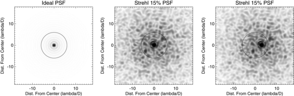
Figure 4. Imaging an unresolved target through a pinhole. The PSF of three targets is shown with a pinhole of size 6λ/D overlaid. Square root contrast scaling is used to highlight the truncated flux. Left: the pinhole, located in an image plane, truncated the portion of electric field which forms the outer rings of the PSF. In perfect seeing, the total flux blocked is very low. Center: wavefront errors dispel flux outward creating a diffuse halo around the target. The blocked flux increases, and more power aliases back into sub-aperture scales, resulting in closure phase errors. Right: when asymmetrically truncated, the center of light shifts toward the pinhole center (black ×). Each component of a binary is truncated differently, leading to errors in astrometry or contrast.
Download figure:
Standard image High-resolution imageAs the PSF varies, so too will the aliased phase errors. This introduces a stochastic component to the closure phase errors which appears to undercut the effectiveness of the pinhole. A portion of the phase errors will also remain fixed and be strictly a function of the asymmetrical truncation of the target and its mean PSF. The latter we term misalignment error to distinguish it from other calibration components. Generally speaking, both will increase as the target is positioned further from the pinhole center.
Qualitatively, we can illustrate that the asymmetrical truncation of the target shifts the visibility and closure phase. Consider Figure 4(c). The visibility phase is influenced by the position of the target on the sky; the asymmetrical truncation of the target shifts its center of light, and so too the visibility phase. While closure phases are normally invariant to the position of the target, the pinhole breaks this invariance. The overall isotropy of the PSF and circular pinhole shape suggests that the misalignment error is symmetric about the origin. That is, just as aligning the target at two diametrically opposed positions will induce equal and opposite shifts in the center of light, the overall symmetry suggests equal and opposite phase errors as well.
The aliased phase errors are small as long as the majority of the flux resides within the pinhole and only competes with the closure phase measurements if the power aliases back into sub-aperture scale wavefront deviations. For this reason, shorter wavelengths will be preferentially advantaged due to their small PSF, assuming that the Strehl ratio is the same at each wavelength. Typically, AO residuals will also be larger for shorter wavelengths (producing a more substantial halo) and this partially counteracts the shorter wavelength advantage. More generally, this suggests that to minimize aliasing, the pinhole could be optimized to filter only frequencies that are not corrected by the AO system; in that case the pinhole size would be matched the AO actuator size instead of the masking sub-aperture size.
Each target of a binary will be truncated differently. The misalignment error can be calculated directly by replacing the single-star PSF in Equation (2) or Figure 4 with the binary image. This will be approximately the same as the error of each component individually. In other words, the misalignment error of the primary added to the misalignment error of the secondary multiplied by the secondary–primary contrast ratio. Assuming that the misalignment error is point symmetric about the origin, aligning the binary center of light near the pinhole center appears to be a viable strategy for minimizing the misalignment error.
If the misalignment component is large enough as to become the limiting component in closure phase noise, there are three approaches which can be employed for removing the component from science data. Empirically, the component can be calibrated by observing a single star aligned at the same location as the primary under similar AO performance. In practice, this may be limited by the accuracy with which one can repeatedly (visually) align a target within the pinhole, and the component arising from the (unknown) companion remains. Computationally, if the location of the primary is known along with an estimate of the PSF, then the misalignment component can be included in the mathematical closure phase model that is fit to data. This approach requires a direct image of the primary within the pinhole to determine its location and estimate its PSF. Both may detract from the overall efficiency of observing. Finally, a third option is to take several sets of aperture masking data with the target (center of light) at various alignments (i.e., dithering) close to the pinhole center. Specifically, if diametrically opposed alignments have misalignment errors opposite in sign, then the component could be averaged out.
2.4. Post-processing with a Window Function
In this course of our investigation of the pinhole filter, we also characterize the use of a tapered window function on masking images to reduce the impact of various noise sources and small-scale wavefront errors on closure phases. For example, we use a super-Gaussian function, exp (− kx4), with our experiments for its flat-top and quickly tapering Fourier transform. For concreteness, we will use this same function as an illustrative example here (Figure 5). The window function is described by the size of its half-width at half-maximum (HWHM) measured in pixels on the detector or in units of λ/D.

Figure 5. Effect of a window function. Top left: the aperture mask produces a set of interference fringes beneath an envelope of size λ/dsub, as seen in this Palomar nine-hole masking image. The central peak has been zeroed to highlight the envelope and outer rings. The radius of the white ring is λ/dsub. Bottom left: the power spectrum of the same interferogram, presented in units of baseline/D rather than spatial frequency. Each island of transmitted power (or splodge) is of size 2dsub. This is expected, as the transmission function is related to the autocorrelation of the mask. Top right: using a window function of characteristic HWHM λ/dsub (here, a super-Gaussian) removes the interferogram wings and its associated read and wavefront noise. Bottom right: the window function produces a convolution kernel of size λ/2HWHM. Note that a window function larger than 0.5 λ/dsub creates a kernel larger than 2dsub and mixes neighboring splodges, adding redundancy noise (see the text).
Download figure:
Standard image High-resolution imageMultiplying the images by a window function that retains the intensity of the interferogram core but tapers at its edges greatly reduces the contamination of detector read noise and dark current, or scattered light from nearby targets not of scientific interest. Per-pixel Gaussian-distributed read noise, when Fourier transformed, results in a per-baseline Gaussian-distributed uncertainty. The per-baseline noise has a magnitude that is directly related to the total transmission of the window function. Therefore, a tighter window function removes more read noise.
However, complex visibilities are extracted from the Fourier transform of the image, so the application of a window function is identical to the convolution of the complex visibilities with the Fourier transform of the window function. This mixes the complex visibilities of the baselines and, ultimately, restricts the minimum window function size.
The aperture mask is designed to be non-redundant for baselines extending between the centers of sub-apertures; the finite size of the sub-apertures give rise to islands of transmitted power in the power spectrum, which we call splodges (see Figure 5, bottom left). The splodges of a completely non-redundant mask do not overlap, and hence the separation between neighboring splodge peaks is about 2 dsub. (In practice, some overlap at the splodge edges may be exchanged for better coverage or larger sub-apertures.) Furthermore, neighboring splodges may arise from completely separate pairs of sub-apertures (i.e., separate baselines), and one would not assume any coherence between the baseline phases. For this reason, window functions narrower than about λ/2dsub, or those without quickly tapered Fourier transforms, will mix the incoherent baselines of neighboring splodges and rapidly increase the error of closure phases, similar to redundancy noise.
The optimally sized window function will balance the reduction of read noise with the increase of redundancy noise.
Post-processing with a window function also reduces the impact of small-scale wavefront errors. This is most readily recognized by noting that the outer rings of the PSF encapsulate the high spatial frequency content of the wavefront; removing this flux also removes the high spatial frequency content of the wavefront.
This method of applying a post-processing window function to spatially filter differs in two major ways from implementing an on-telescope pinhole. Applying filtering in post-processing allows easy tailoring of the shape of the window function (including suppression of the tails of its Fourier transform), a task considerably harder with an apodized pinhole. The pinhole, however, filters the wavefront phase noise at each instant; the window function only filters some form of the time-accumulated phase noise.
3. SIMULATED OBSERVATIONS
We have developed an accurate simulation of the Palomar aperture masking interferometry experiment in order to explore the effect of spatial filtering on wide band data and to optimize the pinhole for implementation on the telescope.
The Palomar nine-hole aperture mask has been described previously in Lloyd et al. (2006) and is shown in Figure 1(a). Placed in the pupil plane, the mask has baselines ranging from 0.71 m to 3.94 m and sub-apertures that are 0.42 m in diameter.
As discussed in Pravdo et al. (2006) and Bernat et al. (2010), aperture masking and the implementation of closure phases work most effectively using the short exposure times, when large-scale wavefront errors (be they atmospheric or instrumental) can be regarded as approximately static. The typical aperture masking operation at Palomar uses exposure lengths of 431 ms. Over this timescale, the evolution of the atmosphere produces a highly dynamic wavefront on sub-aperture scales.
3.1. Characterization and Simulation of Palomar's Atmosphere
Studies by Ziad et al. (2004) and Linfield et al. (2001) conducted with the Palomar Testbed Interferometer (PTI) and Hale 200'' Telescope confirm that the atmospheric turbulence power spectrum is approximately Kolmogorov with an outer scale most often within the range 10–50 m. The median-seeing Fried parameter (r0) has been measured to be 9.0 cm at 550 nm, dropping to 3.8 cm during bad, but regularly observed seeing (Dekany et al. 2007).
Advection (wind) speeds drive the evolution of atmospheric structure within the sub-aperture on intervals between 0.1 and 1.0 s. Using measurements of the Palomar atmospheric temporal structure function over four nights, Linfield et al. (2001) derive wind speeds typically less than 4 m s−1. For shorter timescales, the temporal structure function decays exponentially. The characteristic decay time, which scales with λ6/5, has been measured in two surveys to vary between 15–80 ms (Ziad et al. 2004) and 60–150 ms (Linfield et al. 2001) in Ks.
Our simulations assume an outer scale of 50 m and Fried parameter value 9.0 cm, which correspond to 48 cm in Ks and 32 cm in H. We use wind speeds of 5 m s−1 and temporal decay time of 60 ms.
3.2. Numerical Simulation
We generate time-evolved Kolmogorov phase screens following the procedures of Lane et al. (1992) and Glindemann et al. (1993). These phase screens are characterized by three parameters: the Fried parameter of an instantaneous phase screen, the wind velocity which blows the static phase screen across the aperture, and an additional parameter driving the decorrelation of high spatial frequencies between time steps. From this last parameter emerges the exponentially decreasing temporal structure function for short timescales.
A single 431 ms exposure image is constructed by adding 24 sub-images, each of which is an instantaneous snapshot separated in time by 18 ms. We chose this time step to sufficiently sample the atmospheric evolution over relevant timescales: the wind sub-aperture crossing time is 84 ms; the coherence decay time is 60 ms.
The generated images are 512 × 512 pixels, designed to preserve the pixel scale of the PHARO detector. In frequency space, the 5.08 m aperture spans slightly less than 256 × 256 pixels in the Ks band. Phase screens of this size are generated; this corresponds to an inner scale of approximately 2 cm and sub-apertures approximately 450 pixels in area. We repeated several simulations with four times as many pixels and arrived at similar results; from these results we conclude that our simulation is well sampled.
The simulation generates one sub-image for each phase screen using an incoming monochromatic wavefront perturbed by the screen. After passing through the telescope aperture, the wavefront is corrected by AO, then propagates through the spatial filter, the aperture mask, and, finally, forms an image on the detector. We ignore read noise and photon noise. This simulation is similar to that used by Sivaramakrishnan et al. (2001).
We model the AO system as an instantaneous high-pass filter of the form A(k) = 1/(1 + (kc/k)2), with a cutoff imposed by the Nyquist frequency of the actuator spacing, kc = Nact/2D (about 1.4 cycles m−1 at Palomar). This filter is applied to the Fourier transform of the phase screens and accurately reproduces the wavefront residuals observed under optimal operation at Palomar (Dekany et al. 2007). This overestimates the typical AO performance on faint targets, particularly the performance of tip-tilt suppression. To account for this, we apply the following modified AO filter function, which degrades the low spatial frequency AO response:
To include the polychromatic effects, each wide band transmission filter is divided into a number of subintervals (generally four). A monochromatic image is generated for each subinterval (taking into account wavelength-dependent effects), and these images are added to form a single polychromatic sub-image. The sub-images are co-added to create a single 431 ms exposure.
This produces direct imaging Strehl ratios of 40%–50% in the H band and 60%–70% in Ks.
4. THE PALOMAR PINHOLE EXPERIMENT
4.1. Pinhole Implementation on PHARO
The PHARO instrument (Hayward et al. 2001) is especially suited to a pinhole implementation. PHARO has been designed with coronagraphic capabilities, giving access to both a focal plane and a pupil plane before the final focal plane (Figure 3).
The pinhole is placed in the focal plane before the aperture mask. Based on our simulations from the next subsection, a pinhole of angular diameter 0.779 arcsec was installed at the Lyot Stop in PHARO in 2008 June. This pinhole was chosen for optimal use at 1.6 μm (H band), corresponding to an angular size of 12 λ/D. The pinhole is of size 8.7 λ/D at 2.2 μm (Ks band).
4.2. Pinhole Size Optimization
With sub-aperture sizes of 0.42 m, the estimate from Section 2.3 suggests the optimal pinhole size to be D/dsub ≈ 12λ/D. Using the simulation of the Palomar aperture masking experiment described in Section 3.2, we can determine the optimal pinhole size under typical observing conditions.
For various pinhole sizes, we simulated 100 H-band images of a 10:1 binary with companion separation 150 mas under typical Palomar observing conditions, without read noise, and with the primary aligned at the center of the pinhole. Images of a single star were simulated to be used as a calibrator. We analyzed these images both with and without a window function, and calculated the root-mean-squared (rms) residuals of the simulated closure phases fit to a model binary. Figure 6 shows these results for each pinhole size (with window function, solid line; without window function, dashed line). For reference, the rms obtained with no pinhole in place is included as a horizontal line.
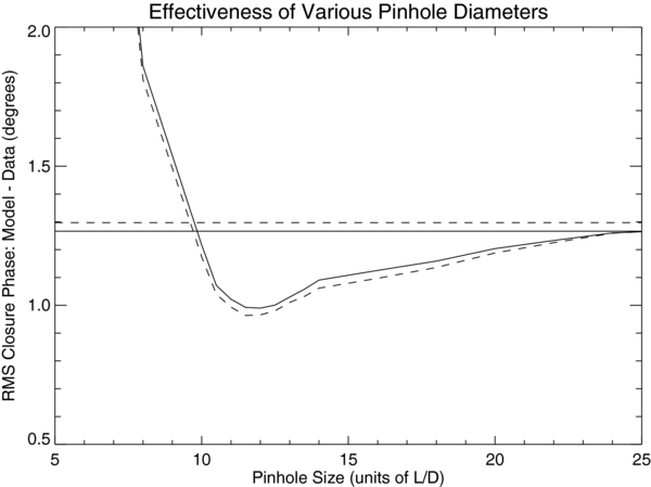
Figure 6. The rms fit residuals of simulated data (AO corrected H-band observing, no read noise) with pinholes of various size, analyzed with (solid line) and without (dashed line) a window function. The model used is an analytic model of closure phase for a single star without noise or wavefront errors. The horizontal line is the measurement level without any pinhole in place. The pinhole filter is most effective within the range 11–14 λ/D.
Download figure:
Standard image High-resolution imageThe spatial filter performance can be broken into following three classes:
- 1.A small pinhole (≲10 λ/D) impinges on the field of view, rejecting enough of the light coming from the off-axis companion so that the closure phases will not match the model. (See also Section 2.3.1.)
- 2.A very large pinhole (≳20 λ/D) provides very little filtering and the data are statistically similar to the unfiltered case.
- 3.The operational pinhole range (10–20 λ/D) reduces the image to image variation of closure phases and produces data that better fit its model. The range 11–14 λ/D is most effective, reducing the fit residuals by roughly 25%.
These results agree with the estimate at the top of this subsection.
Finally, we note that because the window function itself provides some spatial filtering, the inclusion of the pinhole provides slightly less improvement if compared to the case in which no window function is used.
4.3. How Important Is Target Placement?
In Section 2.3.1, we showed that the asymmetrical truncation of the target by the pinhole alters the measured closure phases, even in the absence of wavefront errors, an effect we called misalignment error.
Equation (2) can be directly integrated to determine the misalignment error when a target is observed through the pinhole. Alternatively, we chose to simulate the effect to more accurately reflect the details of our analysis pipeline. For clarity, we present the rms closure phase deviation between the pinhole and non-pinhole values with the Palomar nine-hole mask (averaged over the set of 84 closure phases) in Figure 7.

Figure 7. Misalignment of a single star within the pinhole introduces closure phase errors. (a) The Palomar nine-hole mask, overlaid with three closure triangles for which the misalignment errors are calculated. (b) Error due to misalignment at 1.6 μm (H band) as a function of target distance from the pinhole center. (Several azimuthal orientations are plotted for each separation.) (c) Closure phase errors at 2.2 μm (Ks band) in which the pinhole is smaller. In both cases, errors in visibility amplitude are below 0.005 for the same ranges.
Download figure:
Standard image High-resolution imageBy inspection, we see that in the H band and at high levels of correction (Strehl ≳40%), the pinhole introduces less than 0 3 rms closure phase error at nearly any alignment within the 440 mas diameter pinhole. At a diameter of 12λ/D, less than 2% of the total flux resides outside the pinhole and very little aliases back into the baseline frequencies. The misalignment deviation is also insensitive to the orientation of the misalignment; the aperture mask is three-fold symmetric in physical space, but provides a uniform coverage of spatial frequencies. At moderate Strehl ratios, the misalignment deviation increases, but observationally, this increase is balanced by a larger benefit of spatial filtering.
The alignment requirements are tighter in Ks. Because the pinhole is designed for the H band, its size is only 8.9λ/D in Ks. Good positioning is even more important given that AO residuals and closure phase errors are usually smaller. Alignment can introduce up to 10 of closure phase errors if misaligned by 200–300 mas, or roughly 2–3λ/D.
The presence of a companion adds an additional misalignment error, although this error will be attenuated by the secondary–primary contrast ratio. Therefore, particularly for high-contrast binaries, the misalignment errors provided here give good rule-of-thumb indications of how well a target must be positioned within the pinhole. Given that aperture masking observations at Palomar typically yield 1°–2° of closure phase, targets must be positioned close to the pinhole center during Ks-band observations.
Finally, we note that the percentage of blocked flux is a weak function of the target alignment, and a strong function of the AO performance and size of the direct imaging halo (Figure 7, right panel). In the observations of Section 5 that compare pinhole and non-pinhole observations, the percent loss of flux is a measurable quantity. From the results of this plot, it is clear that large flux drops can be attributed to momentary drops in AO performance or very large shifts in alignment. Astrometric jitter on the scale of hundreds of mas is never seen. Practically, if a series of images contains one or a few with large flux drops, and the target was initially well aligned, then identifying large flux drops is a useful proxy for excluding frames taken with poor AO performance.
4.4. Window Function: Optimal Size and the Palomar Nine-hole Mask
For our experiment, we use a super-Gaussian function, exp (− kx4), for its flat-top and quickly tapering Fourier transform. We describe the window function by the size of its HWHM, wpix, measured in pixels on the detector.
The optimal window function size finds the balance between eliminating read noise and increasing redundancy noise. We present a measure of the effectiveness of various window function sizes in the presence of various levels of read noise in Figure 8.

Figure 8. Window functions reduce closure phase error from read noise. These curves display the reduction of rms closure phase errors by using the ratio of the windowed and non-windowed cases (i.e., the y-axis is a ratio, with 1.0 corresponding to no improvement). These curves, from top to bottom, display the ratio of rms closure phase error when read noise is 0% (top, solid), 0.2%, 0.4%, 0.6%, 1.0%, and 5.0% (bottom, dotted) of the peak image intensity. The optimal window function is typically of size ∼λ/dsub, or ∼12λ/D for the Palomar aperture mask, with higher read noise favoring tighter window functions. Smaller window functions quickly add large amounts of redundancy noise (See the text). Note: even with no read noise (solid curve), a window function reduces closure phase errors, indicating that the window function provides an effect similar to spatially filtering the wavefront.
Download figure:
Standard image High-resolution imageWe simulated 100 images (256 × 256 in size) of a 10:1 binary with companion separation 150 mas and of a calibrator in the same fashion as described in Section 4.2 but without a pinhole in place. To each set of images we added Gaussian read noise with a per-pixel noise level ranging from 0.2% to 5.0% of the peak intensity. (This corresponds to targets of 7th to 10th magnitude when taking 6 s exposures on the PHARO detector.) The images were processed with window functions of various sizes and we calculated the rms residuals of fits to a model binary. In Figure 8, we plot the ratio of the measured rms with a window function to the same set of images without the window function. For all levels of read noise, an optimally sized window function improves the model fits. We caution that, because the effect of read noise on closure phases scales with image size and the choice of default image size is arbitrary, the results can only be evaluated qualitatively.
Several features are apparent. First, the optimal window function is approximately λ/dsub, or ∼12λ/D for the Palomar aperture mask, with tighter windows for the high-noise cases; one expects the optimal window size to be a function of the aperture mask. This makes qualitative sense: the interferogram image is a set of interference fringes under an Airy function envelope of characteristic size λ/dsub. One would expect the optimal window function to crop out those pixels with signal to noise less than one. Beyond λ/dsub, the intensity of the interferogram drops below a few percent of its peak value, comparable to the read noise.
Second, too small a window function quickly adds redundancy noise into the measurements. This turning point is near 0.5 λ/dsub.
Third, even in the absence of read noise, a window function decreases closure phase noise (solid curve). This demonstrates the capacity of the window function to spatial filter the wavefront phase noise, even though the improvement is only about 3%–4%.
To emphasize the utility of the window function as a spatial filter of wavefront errors, we simulated another set of images in which the wavefront is static over the exposure. With only spatial variation of the wavefront, the window function reduces closure phase errors by nearly 20% (Figure 9).

Figure 9. Curves showing the effectiveness of the window function as in Figure 8, except that the wavefront is static over an exposure. Again, these curves display the reduction of rms closure phase errors by using the ratio of the windowed and non-windowed cases (i.e., the y-axis is a ratio, with 1.0 corresponding to no improvement). Most notably, a window function provides better spatial filtering when the wavefront is static (solid line).
Download figure:
Standard image High-resolution imageBy comparing these results to those obtained with an optimized pinhole (25%), it is clear that the pinhole and window functions only provide comparable spatial filtering when the wavefront phase errors is static during an exposure. When accounting for the more realistic, dynamic wavefront, the pinhole provides superior spatial filtering.
Misaligning the peaks of the window function and interferogram introduces a tiny amount of closure phase error. Even an unrealistic misplacement of 10λ/D (about 26 pixels on PHARO at 1.6 μm) with a tight window of size 0.7 λ/dsub produces an error below 006. This will likely be relevant for observations taken by space telescopes.
5. OBSERVATIONS
Between 2008 June and 2009 September, we observed 26 single-star targets and 4 known binaries spanning infrared magnitudes between 6.0 and 9.0 using the PHARO instrument on the Hale 200'' Telescope at Palomar Observatory.
Each aperture masking observation was conducted with and without the pinhole in place to compare the effectiveness and practicality of using the pinhole filter during ground observing. An observing sequence consisted of sets of 20 images (6 second exposures) with the Palomar 9-hole aperture mask in several standard infrared bands. Typically, images were taken in a particular band with the pinhole in place, then again with the pinhole removed, until the sequence of bands had been taken. Similar observations of a calibrator were then taken. This was done to minimize changes in seeing between comparison observations and to minimize the effect of instrumental wavefront changes from slewing the telescope on calibration. Care was taken to use identical detector configurations (position, etc.) and to align the target center of light at the center of the pinhole. This alignment procedure added approximately two to five minutes additional overhead to each observation set.
The aperture mask, data taking procedure, and custom IDL pipeline to analyze aperture masking images have been previously described by Lloyd et al. (2006), Kraus et al. (2008), and Bernat et al. (2010). The mean and variance of the closure phases and amplitudes were calculated (across the set of images) and calibrated. The calibrated closure phases were found by subtracting the calibrator closure phases from those of the target; their errors were estimated by adding in quadrature the errors of the targets and calibrator. The closure phase signal of a single star is zero; deviations from zero may indicate the presence of a companion or result from wavefront errors. The log-amplitudes are calibrated identically and are included to determine if spatial filtering improves measurement of the amplitudes, but are not used for the analysis of the binary candidates. Companions are located by fitting the closure phase data set with a three-parameter binary closure phase model (separation distance, position angle, and contrast ratio) to minimize χ2.
The targets are bright enough that the per-pixel read noise is at or below a few percent. For the analysis that follows, we use the results of Section 4.4 and a window function with HWHM of 1.0 λ/dsub (30.9 pixels in the H band, 41.5 in the Ks band).
5.1. Pinhole Stability and Target Alignment
Images of the pinhole were taken at several periods throughout the run from which its location on the detector can be measured. The location of the pinhole remained accurate to less than two pixels for the entire run, with the exception of two instances in which the Slit wheel appeared to lodge the pinhole at an alternative location. This was easily repaired by putting the Slit wheel into its "HOME" position.
Explicit (direct) images of the target within the pinhole were taken only rarely. However, the locations of the interferogram centers provided an accurate location of the binary targets on the detector. Drift of the target was typically less than one-half pixel during a set of 20 images (about 2 minutes). Comparison of the target and pinhole locations indicate that our alignment was accurate to within four pixels of the measured pinhole center. We conclude that the largest potential source of misalignment error arises from the initial pointing accuracy within the pinhole, and not jitter of the target or pinhole during data taking.
The effect of the pinhole was seen to alter several observables. Most directly, when observing reference stars, the pinhole induced a drop of target flux by roughly 35% in H and 15% in Ks. The pinhole is located after the AO system in the focal plane, hence these values reflect the percentage of the direct imaging PSF which falls outside the pinhole. These percentages are consistent with the pinhole size and the level of AO performance (Strehl ratios of approximately 10% in H and 30% in Ks). Binary targets show a similar drop in flux despite their larger size, which we can take as an indication that their center of light is well aligned.
Simulations and calculations using a sample of direct images show that the percentage of blocked flux is a weak function of the target alignment, and so large flux variations do not indicate a high level of astrometric jitter. Instead, this percentage is a strong function of the AO performance (and size of direct imaging halo). Low transmission (below 40%) well identified individual images blurred by temporary drops in AO correction. High flux transmission well predicted good fits to models (e.g., Figure 10).
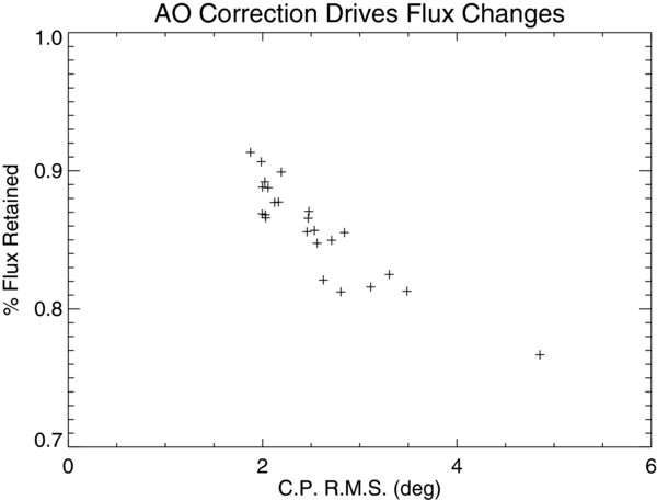
Figure 10. Drops in flux transmission through the pinhole are driven by changes in the PSF, which are tied to AO performance. The binary GJ 623 was resolved in Ks using 25 masking images through the pinhole. The images that produced the best-fitting closure phases (as measured by rms deviation from the model) also had the least flux blocked by the mask. Poor correction (lower Strehl ratio) displaces more flux into the outer halo of the PSF, which is then blocked by the pinhole. Poor correction also leads to larger closure phase errors. Thus, these two effects are strongly correlated. This trend is not caused by misalignment or movement of the target within the pinhole (see the text), but rather changes in AO correction (and lower Strehl ratio).
Download figure:
Standard image High-resolution image5.2. Calibrators: Pinhole Filtering Produces Lower Closure Phase Variance and Higher Amplitudes
The use of the pinhole generally reduced the variance of closure phases and increased the amplitudes for the observed single stars. These results are compared to a set of simulated observations in Figure 11.

Figure 11. Closure phase standard deviation (scatter) is reduced and baseline visibility amplitude is increased when observed through the pinhole filter. Data points are drawn from observations of 26 single stars. Horizontal lines are the median of the data (solid) and the simulated experiment (dashed). Top row: closure phase scatter is reduced by 10% and 19% in H- and Ks-band measurements, respectively. Bottom row: visibility amplitude is increased by 14% and 18% in H and Ks bands, respectively. In all cases, the simulation (model) predicts a larger reduction in noise (see the Discussion).
Download figure:
Standard image High-resolution image
The closure phase standard deviation is reduced by 10% and 19% in the H band (1.6 μm) and the Ks band (2.2 μm), respectively. A larger reduction is expected at the longer wavelength, as the pinhole is relatively smaller and provides more aggressive spatial filtering. Although not displayed, the rms residuals of the data fit to their model values also reduced by 10%–20% indicating better calibrated data. The pinhole filtering increases the visibility of log-amplitude by 14% and 18% on the longest baselines at the H band and the Ks band, respectively. Each of these confirm that the spatial filter is reducing closure phase noise from sub-aperture redundancy.
In both cases the simulation predicts a larger reduction in variance, although the results across wavelengths are consistent. The simulation does not include the time-variation of AO residuals during a single exposure, particularly slow tip-tilt correction of the PALAO system (Bloemhof et al. 2001). This can produce several interferograms in a data set with large closure phase errors which cannot be improved by spatial filtering.
5.3. Binaries: Lower Closure Phase Variance
We observed four previously characterized binaries with well-defined orbits with and without the pinhole in several bandpasses: GJ 164 (Martinache et al. 2009), G 78-28 (Pravdo et al. 2006), GJ 623 (Martinache et al. 2007), and GJ 802B (Ireland et al. 2008). The characterized orbits were used to predict the location of each companion on the observing date using a Monte Carlo simulation to account for the uncertainty of the orbital parameters. Each target was observed to obtain 20 images (6 second exposures) in several bandpasses in 2009 September. Three of the four known binaries were successfully resolved (Table 1). The high-contrast companion to GJ 802B could not be resolved at the correct separation and contrast ratio. The quality of each set can be quantified by the rms of the difference between the data closure phases and the best-fitting closure phase model of a binary. The astrometry of the best-fitting binary model can also be compared to the astronomy predicted by the orbital parameters in the literature.
Table 1. Observation of Known Binaries with and without Spatial Filter
| Binary | Band | Separation | Position Angle | Contrast | Best-fit | Median | Cal | Estimated | Estimated |
|---|---|---|---|---|---|---|---|---|---|
| (mas) | (°) | Δ Mag | rms (°) | σϕ(°) | ϕsys(°) | σalign(°) | |||
| GJ 164 | H | 48.7 ± 1.9 | 346.5 ± 1.7 | d | 4.03 | 2.11 | Y | 3.4 | |
| H (SPF) | 48.8 ± 1.5 | 343.9 ± 0.9 | d | 3.33 | 1.99 | Y | 2.7 | 0.61 | |
| Predicteda | 49.4 ± 2.2 | 348.1 ± 10.1 | 1.835 ± 0.006 | ||||||
| Ks | 46.8 ± 1.2 | 340.3 ± 1.0 | d | 3.46 | 1.20 | Y | 3.2 | ||
| Ks (SPF) | 46.3 ± 0.7 | 341.2 ± 1.2 | d | 2.16 | 0.70 | Y | 2.9 | 0.42 | |
| Predicteda | 49.4 ± 2.2 | 348.1 ± 10.1 | 1.721 ± 0.097 | ||||||
| G 78-28 | H | 101.7 ± 0.3 | 359.2 ± 0.2 | 1.275 ± 0.010 | 2.78 | 1.16 | Y | 2.5 | |
| H (SPF) | 102.6 ± 1.4 | 359.6 ± 0.2 | 1.323 ± 0.015 | 3.00 | 1.09 | Y | 2.8 | 0.68 | |
| Predictedb | 105.0 ± 5.7 | 359.3 ± 1.8 | 1.24 ± 0.07 | ||||||
| Ks | 103.4 ± 0.3 | 359.0 ± 0.1 | 1.221 ± 0.007 | 2.68 | 0.72 | Y | 2.6 | ||
| Ks (SPF) | 104.5 ± 0.2 | 359.3 ± 0.1 | 1.221 ± 0.005 | 3.60 | 0.56 | Y | 3.6 | 0.75 | |
| Predictedb | 105.0 ± 5.7 | 359.3 ± 1.8 | 1.14 ± 0.06 | ||||||
| J | 101.4 ± 0.6 | 358.7 ± 1.3 | 1.257 ± 0.021 | 7.60 | 3.12 | Y | 6.9 | ||
| J (SPF) | 100.8 ± 0.6 | 358.5 ± 0.2 | 1.263 ± 0.011 | 5.80 | 2.55 | Y | 5.2 | 0.24 | |
| Predictedb | 105.0 ± 5.7 | 359.3 ± 1.8 | 1.24 ± 0.07 | ||||||
| GJ 623 | CH4s | 282.3 ± 1.4 | 176.3 ± 0.4 | 2.798 ± 0.050 | 3.38 | 1.90 | N | 2.8 | |
| CH4s (SPF) | 277.3 ± 3.0 | 176.2 ± 0.2 | 2.829 ± 0.51 | 3.43 | 1.65 | N | 3.0 | 0.75 | |
| Predictedc | 279.1 ± 1.2 | 177.4 ± 0.7 | 2.860 ± 0.039 | ||||||
| Ks | 277.1 ± 0.4 | 176.5 ± 0.1 | 2.675 ± 0.014 | 2.35 | 0.45 | N | 2.3 | ||
| Ks (SPF) | 280.7 ± 0.2 | 176.6 ± 0.7 | 2.780 ± 0.10 | 1.9 | 0.30 | N | 1.9 | 0.46 | |
| Predictedc | 279.1 ± 1.2 | 177.4 ± 0.7 | 2.720 ± 0.014 | ||||||
| Brγ | 279.1 ± 0.3 | 176.2 ± 0.7 | 2.664 ± 0.012 | 0.94 | 0.42 | N | 0.8 | ||
| Brγ (SPF) | 279.4 ± 0.4 | 176.5 ± 0.1 | 2.778 ± 0.009 | 1.28 | 0.33 | N | 1.2 | 0.63 | |
| Predictedc | 279.1 ± 1.2 | 177.4 ± 0.7 | 2.720 ± 0.014 | ||||||
Notes. Measurements of three known binary systems with and without the pinhole filter (SPF). aSpatial filtering reduces the median scatter of closure phase measurements in all cases. bThe median residual between the data and best-fitting model does not increase when using the pinhole. cAn estimate of the systematic error due to a misalignment of 3 pixels. See the text for discussion. dThe target GJ 164 data were fit to a binary model holding fixed the mean contrast ratio given by Martinache et al. (2009). Note: Target GJ 802 is excluded from this table.
Download table as: ASCIITypeset image
GJ 164 was imaged for three sets near dawn with the pinhole and one set without. All but the first sets of data suffered poor AO correction, were visibly less sharp, and had flux levels drop by nearly 75%. The binary could be well resolved in all three sets with the pinhole, but the latter sets yield much worse fits and larger systematic errors and are not used in the analysis. The fit parameters to GJ 164 share a degeneracy with a spurious set of parameters (ΔH = 0.030, at nearly the same location), and limit the quality of parameter errors which can be derived from the fit. Instead, the magnitude contrast was held fixed to the values determined by Martinache et al. (2007). The observations of reference stars to calibrate GJ 623 varied in AO correction and quality between pinhole and non-pinhole measurements, and so this target is presented without calibration in order to compare the two performances.
The median closure phase scatter (stochastic errors) decreased for each observation by roughly 20%–25%, which indicates that the pinhole operated effectively to minimize closure phase errors from AO residuals. However, the data fits to binary models showed no decrease in rms residuals, whereas the fits to single-star data decreased by 10%–20%. Of the eight total measurements, four showed an increase in rms, although only two Ks-band observations increased by more than 10%. The observations that increased in rms are those in which either the companion was aligned far from the pinhole center or the companion is comparatively bright. We prefer to discuss this measurement in terms of the amount of unattributed systematic error that needs to be added in quadrature to the stochastic errors to yield the rms values, i.e., (rms)2 = 〈σ2ϕ + σ2sys〉. This is listed in the next to last column of Table 1. A systematic component of 10 specific to binary targets would account for the discrepancy of performance.
Misalignment of the target within the pinhole contributes to the increased residuals. Because each binary system could be resolved by direct imaging, the targets were aligned with their center of light as close to the pinhole center as could be accurately judged by eye. This necessarily placed each star off-center of the pinhole. The astrometric alignment of each component can be inferred from the center of the interferograms and is listed in Table 2. As discussed earlier, the alignment of the components is determined by the original placement of the observer and moves comparatively little during a set of images.
We simulated each binary with and within the pinhole displaced by the amounts in Table 2. The atmospheric seeing was tuned to fit Strehl ratio estimates from direct images taken throughout the night: 40% in Ks and Brγ bands, 15% in H and CH4s bands, and 10% in the J band. The astrometric jitter of the simulated images was consistent to those observed (and less than 20 mas per 20 images for most targets). Each simulation produced enough images until all errors reached a steady state; the estimates of the misalignment error are included in the last column of Table 1. Additional contributions from misaligned calibrators are not included.
Our calculation of the misalignment error requires knowledge of the absolute positions of the pinhole and target components, and an accurate measure of the PSF. Given the small jitter of targets, our calculation is limited by imperfect knowledge of the PSF. Even still, the quality of correction can fluctuate in timescales of minutes, as can be observed by viewing successive direct images or other observables such as pinhole transmission (Figure 10). Given these assumptions, misalignment contributes systematic components of 04–08 to the H- and Ks-band binary observations. We also note that simulations demonstrate large ≳ 10 alignment errors for slightly lower Strehl ratios (≲10% in H and ≲20% in Ks). These challenges instead warrant the development of an observing strategy to calibrate alignment errors empirically.
The binary parameters measured with and without the pinhole, and those predicted by the system orbits, are in good agreement. In each case, the spatial filter data fit to slightly higher contrasts ratios (≈5%). This may indicate that the companion flux was skewed closer to the pinhole edge and its flux truncated by a few percent more, which is consistent with the measured locations of the objects within the pinhole (Table 2). No bias was found in the relative astrometry.
Table 2. Astrometry and Alignment of Targets within Pinhole
| Distance From Center (mas) | Estimated | |||
|---|---|---|---|---|
| Binary | Band | Primary | Secondary | σalign |
| GJ 164 | H | 90 ± 50 (60) | 140 ± 50 (60) | 0.61 |
| Ks | 50 ± 15 (40) | 90 ± 15 (40) | 0.42 | |
| G 78-28 | H | 90 ± 35 (50) | 110 ± 35 (50) | 0.68 |
| Ks | 80 ± 10 (40) | 70 ± 10 (40) | 0.75 | |
| J | 100 ± 25 (45) | 170 ± 23 (45) | 0.24 | |
| GJ 623 | CH4s | 130 ± 10 (35) | 200 ± 10 (35) | 0.75 |
| Ks | 90 ± 10 (40) | 200 ± 10 (40) | 0.46 | |
| Brγ | 150 ± 10 (40) | 190 ± 10 (40) | 0.63 | |
Notes. Alignment of targets within pinhole and estimated closure phase misalignment error. Position determined by center of interferograms; errors estimated from spread over 20 images. Values in parentheses include 40 mas uncertainty of the absolute pinhole position. Misalignment errors are calculated using the simulation of Section 4.3, assuming a Strehl of 15% in H and CH4s, 45% in Ks and Brγ, and 10% in the J band.
Download table as: ASCIITypeset image
Generally speaking, the lower closure phase errors brought on by the pinhole filter ought to lead to proportionally lower errors in binary parameters and higher contrast of detection. The pinhole demonstrably decreases closure phase measurement error by 20%–25% and indicates that, if the systematic component can be minimized, the pinhole can provide an increase of contrast by 20%–25% using the same length of observation. However, the misalignment error limits the increase in precision. In practice, we scale the closure phase measurement errors until the χ2 of the best fit is unity to account for any known systematic errors. Therefore, to maintain the increased precision in this analysis, the decrease in closure phase measurement error must be matched by a similar decrease in rms fit residual (or systematic component). Since the fit residuals did not improve, the precision in the binary parameters did not improve in all cases.
6. SUMMARY OF RESULTS AND CONCLUSIONS
In this text, we discussed spatial wavefront variation on the scale of NRM sub-apertures, which contributes to closure phase errors we called sub-aperture redundancy noise. We proposed that quasi-static wavefront errors on the scale of the sub-aperture, which evolve over hundreds of seconds or with telescope movement, give rise to the limitations of aperture masking calibration. Through simulations and direct observation we have shown that the use of a pinhole filter effectively reduces sub-aperture spatial variation and can reduce closure phase errors, increase visibility amplitudes, and lead to better calibration and higher detection contrasts.
With a simple premise, we estimate the optimal pinhole size to be dspf ≈ D/dsub in units of λ/D, or about 12λ/D for the Palomar nine-hole mask. We confirm this result using a detailed simulation of the Palomar aperture masking experiment and show that the operational pinhole size ranges from 11 to 14 λ/D. Smaller pinholes reject enough light from off-axis companions to alter the measured closure phases. Larger pinholes provide little spatial filtering.
Because the pinhole is not a perfect low-pass filter, the truncation of off-axis targets aliases power back into phase at sub-aperture scales. This introduces closure phase errors of its own, both systematic and stochastic. Using simulated observations over a wide range of corrections (Strehl ratio of 10%–100%), we show that a misalignment of the target by 200 mas introduces 03–10 of systematic closure phase, which we have termed misalignment error. We propose several methods for the calibration of this component although none are undertaken in this experiment. As a result, the effectiveness of pinhole technique is limited by the accuracy with which targets can be aligned within the center of the pinhole.
We installed a pinhole of size 0.779 arcsec (12λ/D at 1.6 μm) in the Slit wheel focal plane of the PHARO instrument on the Hale 200'' Telescope at Palomar Observatory. Using this pinhole we observed twenty single unresolved stars and three well-characterized binaries with and without the pinhole in a selection of standard near-infrared bands. The AO system provided moderate corrections: Strehl ∼5%–15% in the H band and ∼20%–40% in the Ks band.
Observations of unresolved stars showed that the pinhole reduced the stochastic variation of closure phases by 10%–25% from one image to the next, and visibility amplitudes increased. rms residuals to model fits decreased by a similar factor. Each shows that increasing sub-aperture coherence decreases closure phase redundancy noise. Lower fit residuals indicate that calibration improved, and that the aperture masking calibration limit is partially attributable to small-scale quasi-static wavefront errors. Furthermore, detection contrasts scales proportional to fit residuals, indicating an increase in detection contrast of 10%–25%.
The modest increase in closure phase signal to noise when the pinhole is used suggests that the spectrum of wavefront errors contains relatively little power on the smallest spatial-scales within the sub-aperture. Additionally, the smallest scale variations that cycle multiple times within a single sub-aperture tend to produce redundancy noise that averages out. The leading source of spatial redundancy noise, both quasi-static instrumental and residual atmospheric wavefront errors, is more likely low-order Zernike modes (i.e, "phase slopes") across the sub-apertures.
Simulations of these observations, when compared, predict a slightly larger benefit from the pinhole filtering. As discussed in Section 2.2, temporal variations of the baseline phase within a single exposure lead to a sort of temporal redundancy noise that cannot be removed by closure phases of the pinhole filter. Furthermore, the slow response of the Palomar AO tip-tilt mirror (5 Hz) gives rise to full aperture scale wavefront residuals which evolve on the order of a fraction of an exposure. The baseline phase changes these residuals induce contribute to the overall variation of the closure phases from one image to the next (though not calibration errors). The simulation did not include temporal variations of the AO residuals, and as a result gives the impression that the pinhole is more effective at reducing stochastic closure phase noise (50% versus 20%). Indeed, these results imply that temporal variation of the wavefront phase is a large source of closure phase variance with the current PALAO system.
We observed three well-characterized binary systems to determine how the pinhole influences the astrometric and photometric characterizations of discovered systems. The measured binary parameters were consistent with those acquired without the pinhole and those predicted by the measured orbital parameters of the system. No bias was found in the astrometry (i.e., binaries did not tend toward shorter separations with the pinhole); however, contrast ratios with the pinhole tended to be a few percent fainter. Our alignment technique placed the system center of light near the pinhole center, and the light of the companion is preferentially blocked by this arrangement. Better positioning of the target would likely remedy this bias.
Although closure phase stochastic errors decreased by 20%–25%, binary data acquired with the pinhole provided no better fits to data and suggest that binary targets observed with the pinhole contain an additional 10 systematic error. After simulating these observations with and without the pinhole, we conclude that the systematic component arises from the off-center alignment of a resolved target. Simulations demonstrate large ≳ 10 alignment errors at low Strehl ratios (≲10% in the H band and ≲20% in Ks).
Binary parameter errors and detection contrast both decrease in proportion to the closure phase errors, and indicate that one can achieve more precisely measured binary parameters and higher contrasts (20%–25%) with the pinhole.
Finally, we showed that multiplying the images by an apodized window function acts to reduce the effects of wavefront error similar to a spatial filter. Applying this post-processing method for spatial filtering allows easy tailoring of the shape of the filtering function, but only filters some form of the time-accumulated wavefront phase noise (not instantly). We found that the optimal window function has a HWHM of about λ/dsub, with smaller window functions favored for targets in which read noise is higher. By comparing the results of the two methods, it is clear that on-instrument filtering is superior because of the substantial temporal variation of the wavefront phase noise on sub-aperture scales.
7. DISCUSSION
7.1. A Strategy for Future Pinhole Observations
In light of this investigation, the pinhole can prove to be effective in two scenarios. When seeing or correction is poor, and closure phase observations do not reach the calibration limit, a pinhole filter will clearly provide higher signal-to-noise closure phases and more efficient data taking.
At the other extreme, the pinhole may be valuable for improving very high Strehl ratio (≳80%) observations with extreme-AO systems. The high spatial frequencies filtered by the pinhole contribute to a larger proportion of the overall wavefront errors in this scenario. The pinhole could be optimally tuned to the AO actuator size, much larger, and alignment requirements would be substantially relaxed. Most importantly, the aliasing of high spatial frequency content into sub-aperture scale phase errors is a higher order effect of the wavefront (Poyneer & Macintosh 2004). At very high levels of correction, the aliased power is a smaller component of closure phase errors.
We can arrive at a rough estimate of a pinhole performance on extreme-AO systems by simulating a higher-order AO system, such as the 3368-actuator Palomar 3000 system (P3K; Dekany et al. 2007). As mentioned earlier, our simulation does not account for the sluggish tip-tilt correction of the current Palomar system and overpredicted the pinhole performance as a result. The P3K system will have upgraded response by using the current 241 actuator system to perform low-order correction, and thus provide more stable correction. Using the specifications of this system, we simulated a 10:1 binary separated by 150 mas in the H band under typical conditions (see Section 4.2). A pinhole of size 12λ/D decreased stochastic closure phase errors to 20% nominal values, i.e., a five-fold increase in signal to noise. When compared to our simulations of the current AO system (a two-fold increase), the pinhole can impact extreme-AO observations favorably.
For very high Strehl ratio observations, misalignment error will be lower and less sensitive to changes in correction (019 in this example). Empirically calibrating misalignment by observing a reference star at the same position as the primary is only a partial solution (as it does not take into account the companion), likely limited by the pointing accuracy of the observer, and decreases the overall efficiency of the observations. Instead, observations should be taken by dithering the center of light around the pinhole center to minimize this systematic component. Using diametrically opposed target placements successfully reduced the misalignment component to 011 in simulation, a reduction of nearly half.
Finally, one must also consider the optimal pinhole size to survey across the near-infrared bands. For example, if the effective range of pinhole sizes is narrow enough (e.g., 11–14 λ/D for this experiment) a single pinhole may not accommodate multiple wide band infrared filters. In those cases, multiple pinholes tuned to specific observation bands will be most effective.
7.2. Extreme-AO Aperture Masking Experiments
Next generation AO systems with aperture masks, such as Palomar 3000 (Dekany et al. 2007) and Gemini Planet Imager (Macintosh et al. 2008), provide actuator densities high enough to correct wavefront errors on sub-aperture scales. Design and optimization of these aperture masking experiments that balance sub-aperture size and number against AO correction and the limitations of systematics require a more detailed understanding of how sub-aperture wavefront errors impact closure phases, and where resources should be focused. Extreme-AO systems are anticipated to provide highly stable correction down to scales of 8 cm and thus may motivate smaller and additional sub-apertures, providing more spatial frequency coverage and resolution. This balance will depend on the spatial and temporal power spectra of the corrected wavefront residuals. These data should be accumulated and their impact on closure phase errors should be examined.
We thank the staff and telescope operators of Palomar Observatory for their support and many nights of assistance at the Hale Telescope. The authors appreciate the effort of the reviewers, who provided valuable advice on the clarity and depth of this text. This material is based upon work supported by the National Science Foundation under Grant No. AST-0705085. The Hale Telescope at Palomar Observatory is operated as part of a collaborative agreement between Caltech, JPL, and Cornell University. This publication makes use of data products from the Two Micron All Sky Survey, which is a joint project of the University of Massachusetts and the Infrared Processing and Analysis Center/California Institute of Technology, and is funded by the National Aeronautics and Space Administration and the National Science Foundation.
Facility: Hale - Palomar Observatory's 5.1m Hale Telescope
APPENDIX: PINHOLE FILTERING: INTEFEROMETRY
Observing through a pinhole alters the measured complex visibility of a point source even in the absence of any wavefront aberrations. This analysis assumes that the Fraunhofer approximation applies, i.e., that the electric field in the image plane is the Fourier transform of the phasor of the wavefront phase in the pupil frame. We assume no wavefront aberrations, including those from optical errors and central obscurations.
The optical path is shown in Figure 3. We denote the electric field at the telescope aperture with the subscript a and the electric field after spatially filtering with the subscript spf. The coordinates in the image plane are  ; all angles are measured in units of λ/D. We assume that the pinhole has angular diameter dspf and is positioned at
  . The point source is located at an angular position
  on the sky and
  corresponds to perfect alignment of the source in the pinhole.
The wavefront phasor at the entrance of the aperture is
The optics of the spatial filter truncate the electric field in the focal plane, which results in a convolution when the field is transformed back at a pupil plane. The spatially filtered electric field is then
where the star represents convolution.
The use of an aperture mask,  , containing a baseline
  ultimately measures the spatial frequency
  of the complex visibility. For clarity, we present this as a function of baseline:
where  is the electric field sampled by the mask.
Without the spatial filter, substitution for the field from Equation (A1) gives
With the spatial filter, the aperture mask samples  of Equation (A2). By recognizing that convolution with
  leads to a Fourier transform, doing so before substitution yields
In the limit of an infinite pinhole, the integral converges to the value  .
.
We can extend use of this approach to include arbitrary pupil-plane phase errors which arise prior to propagation through the pinhole system. In the presence of inhomogeneous phase in the pupil plane, eiϕ(x), Equation (A2) becomes
Repeating the steps above, the complex visibility is written as
with
Footnotes
- 6
The Jinc function is defined as Jinc(x) ≡ (J1(x)/x). It is the two-dimensional Fourier transform of a circular aperture and is related to the Airy function by Airy(x) = 4 Jinc(x)2.