


ABSTRACT
We study archival HST [S ii] 6716+30 and Hα images of the HH 34 outflow, taken in 1998.71 and in 2007.83. The ∼9 yr time baseline and the high angular resolution of these observations allow us to carry out a detailed proper-motion study. We determine the proper motions of the substructure of the HH 34S bow shock (from the [S ii] and Hα frames) and of the aligned knots within ∼30'' from the outflow source (only from the [S ii] frames). We find that the present-day motions of the knots along the HH 34 jet are approximately ballistic, and that these motions directly imply the formation of a major mass concentration in ∼900 yr, at a position similar to the one of the present-day HH 34S bow shock. In other words, we find that the knots along the HH 34 jet will merge to form a more massive structure, possibly resembling HH 34S.
Export citation and abstract BibTeX RIS
1. INTRODUCTION
Reipurth et al. (1986) showed that HH 34 has a remarkable, jet-like chain of knots (extending southward ∼30'' away from the source), pointing toward an extended bow shock (HH 34S, at ∼100'' from the outflow source). Further observations showed the presence of a northern bow shock (HH 34N, with remarkable point symmetry with respect to HH 34S) and a sequence of bipolar bow shock pairs at larger distances from the source (Bally & Devine 1994; Eislöffel & Mundt 1997; Devine et al. 1997). Recent IR spectroscopic observations (García López et al. 2008) and Spitzer images (Raga et al. 2011b) have also shown the existence of a northern chain of aligned knots, with remarkable knot-to-knot symmetry with respect to the southern knot chain discovered by Reipurth et al. (1986). Spectrophotometry, radial velocity, and proper-motion measurements at optical (see, e.g., Heathcote & Reipurth 1992; Eislöffel & Mundt 1992; Morse et al. 1992, 1993; Reipurth et al. 2002; Beck et al. 2007) and IR wavelengths (Stapelfeldt et al. 1991; Stanke et al. 1998; Reipurth et al. 2000; García López et al. 2008; Coffey et al. 2011) have been carried out. The structure of the HH 34 jet has been modeled as a variable jet with relatively convincing results (e.g., Raga & Noriega-Crespo 1998; Raga et al. 2011a).
In this paper, we carry out a study of proper motions of the southern lobe of the HH 34 outflow based on a comparison of two [S ii] 6716+30 and Hα Hubble Space Telescope (HST) images, obtained at a ∼9 yr time interval. The first [S ii] and Hα frames were described by Reipurth et al. (2002), and the second epoch by Hartigan et al. (2011). The latter paper actually compares the two epochs that we are using, but does not present quantitative proper-motion determinations.
The paper is organized as follows. The observations are described in Section 2. The proper motions of the HH 34S bow shock are presented in Section 3. The proper motions of the knots along the HH 34 jet are described in Section 4. Finally, Section 5 presents a discussion of the results.
2. OBSERVATIONS
In this paper, we analyze HST images of HH 34 obtained at a ∼9 yr time interval (1997–2007). There is also a previous epoch, which we have not used in this paper because it has a significantly lower signal-to-noise ratio.
We have downloaded from the HST archive the [S ii] 6716+30 frames of HH 34 obtained in 1998.71 (with a total exposure time of 13380 s; see Reipurth et al. 2002) and 2007.83 (with an exposure time of 9600 s; see Hartigan et al. 2011), and the Hα frames obtained in 1998.71 (13400 s exposure time) and 2007.83 (9600s exposure time). The two pairs of frames were aligned using the four common stars with the highest signal-to-noise ratio, and the standard IRAF routines GEOMAP and GEOTRAN to measure their positions and shift-and-rotate one of the images (2007) with respect to the other one (1998). Since the astrometry of the individual frames is very good, the corresponding pixel shifts are ∼ half a pixel with an rms error of a tenth of a pixel (of an original 0.1 arcsec pixel−1 in the drizzle images).
We have rotated the images so that the HH 34 outflow axis lies approximately parallel to the ordinate. The region of the 1998.71 [S ii] frame with the HH 34 jet and HH 34S bow shock is shown in Figure 1.
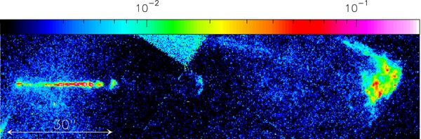
Figure 1. 1998.71 [S ii] 6716+30 image of the southern lobe of the HH 34 outflow. The image has been rotated so that the outflow axis lies approximately parallel to the ordinate. The [S ii] fluxes are shown with the logarithmic scale (in photons cm−2 s−1 pixel−1) given by the top bar. The scale is indicated by the arrow on the bottom left of the image.
Download figure:
Standard image High-resolution imageWe should note that [S ii] and Hα images from a previous epoch (1994) also exist in the HST archive (see Ray et al. 1996). These images have a total exposure time of ∼3000 s, and therefore have a considerably lower signal-to-noise ratio than the other two epochs (with ∼3–4 times longer exposures; see above). We have therefore not included the 1994 frames in our analysis because of their lower signal-to-noise ratio together with their relative proximity in time to the 1998.71 frame. Attempts to include these frames in our analysis do not lead to improved results.
3. THE HH 34S BOW SHOCK
3.1. Proper Motion of HH 34S
Figure 2 shows the rotated and aligned 1998.71 and 2007.83 [S ii] images of the region around HH 34S. We define a 19'' × 21'' box (shown on the two images) including HH 34S, and carry out a cross-correlation of the emission (within this box) of the two epochs.
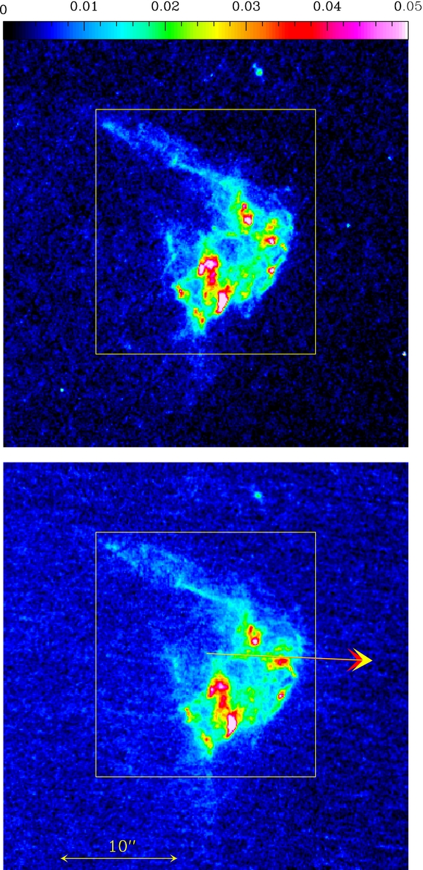
Figure 2. Region around HH 34S in the 1998.71 (top) and 2007.83 (bottom) [S ii] images. The box used for the cross-correlations is shown on the two frames, and the resulting proper motion is indicated in the bottom frame (red arrow: [S ii] proper motion; yellow arrow: Hα proper motion; the red arrow mostly lying under the yellow arrow). The images are depicted with the linear scale (in photons cm−2 s−1 pixel−1) given by the top bar.
Download figure:
Standard image High-resolution imageFrom a paraboloidal fit to the peak of the cross-correlation function, we find a Δx = 0 923 offset along the outflow axis and Δy = −0043. The error resulting from the alignment of the two frames and the fitting to the peak of the cross-correlation function is of ≈002. The observed displacement corresponds to a proper motion of PM34S = (0101 ± 0002) yr−1, corresponding to a plane-of-the-sky velocity vT, 34S = (215 ± 5) km s−1 at a distance of 414 pc (see Menten et al. 2007). An arrow illustrating this motion is shown in the bottom frame of Figure 2.
In an analogous way we have calculated the proper motion of HH 34S from the 1998.71 and 2007.83 Hα images. A plane-of-the-sky velocity of (222 ± 5) km s−1 is obtained, which is not significantly different from the velocity deduced from the [S ii] images (see above). The Hα proper-motion vector is shown in Figure 2.
From the observed proper motion and a distance x34S ≈ 105'' between the source and HH 34S, we obtain a dynamical time tdyn, 34S = x34S/vT, 34S ≈ 1000 ± 50 yr. Therefore, if HH 34S travels ballistically, the ejection velocity had a value vj ≈ vT, 34S/cos 35° ≈ 270 km s−1 (where ϕ = 35° is the approximate angle between the HH 34 outflow axis and the plane of the sky, see Section 4.3) at a time t = −1000 yr (t = 0 corresponding to 2007.83).
3.2. Relative Motions of the Substructures of HH 34S
In order to study the relative motions of the substructure of HH 34S, we first displace the 1998.71 [S ii] image using the proper motion of the whole HH 34S bow shock (see Section 3.1). In this way, we have two images (the 2007.83 map, and the displaced 1998.71 map) in which the cross-correlation of the whole HH 34S structure has a peak at zero displacement.
We now take these two maps and cover them with 24 side square boxes, with displacements of 12 between the centers of the boxes (so that the successive boxes have 12 overlaps). For all of the boxes in which the peak flux in the two images is larger than 0.01 photons pixel−1 cm−2 s−1, we then carry out cross-correlations in order to calculate a proper motion for the emission of the material within the boxes. In this way, we calculate the "kinematical map" shown in Figure 3.

Figure 3. Relative [S ii] proper-motion map of HH 34S (see the description in Section 3.2). Top frame: the arrows show the proper motions (relative to the motion of HH 34S) computed in 24 square boxes. Bottom frame: the central regions of the cross-correlation boxes are shown, and within each of the boxes are written the components of the proper-motion velocities along (top number) and across (bottom number) the outflow axis.
Download figure:
Standard image High-resolution imageKinematical maps such as the one shown in Figure 3 can be computed for arbitrary box sizes. We find that for boxes smaller than ≈2'' an increasing number of spurious proper motions (identified by their disproportionally large values and arbitrary directions) are obtained, particularly in relatively low intensity regions. For larger box sizes, maps similar to the one shown in Figure 3 are obtained, but with a lower angular resolution. In this way, the size that we have chosen for the cross-correlation boxes is close to the smallest size possible for calculating a coherent kinematical map (therefore resulting in about the highest possible angular resolution for the map).
The [S ii] kinematical map (see Figure 3) shows regions with velocities close to zero, indicating that they have a proper motion similar to the average proper motion of the whole HH 34S structure. Not surprisingly, the brighter condensations have relative velocities close to zero (as they are the ones that determine the average motion of HH 34S).
Interestingly, we see that in the region toward the outflow source, we have material with trailing velocities (the largest of these in the extended bow shock wing on the top of Figure 3). Also, there are regions of trailing velocity within the central region of HH 34S. Finally, in the region farthest away from the outflow source, we see a cross-axis expansion motion. These qualitative features of the [S ii] kinematical map are summarized in the schematic diagram shown in Figure 4.
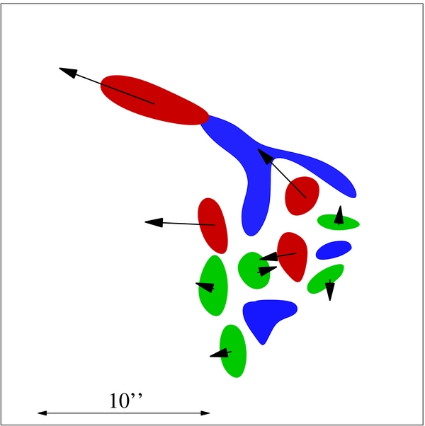
Figure 4. Schematic diagram summarizing the characteristics of the HH 34S relative proper-motion map (see Figure 3). The regions with proper motions <20 km s−1 are shown in blue. The regions with velocities between 20 and 50 km s−1 are shown in green. Finally, the regions with proper motions >50 km s−1 are shown in red. This diagram shows the general structure of trailing motions in the wings and lateral expansion in the bow shock head described in the text.
Download figure:
Standard image High-resolution imageIn Figure 5, we show the relative proper motions which result from the Hα images. As is clear from the top frame, the Hα maps of HH 34S show a structure of superposed "wisps" (described in detail by Reipurth et al. 2002), which differs in a qualitative way from the "clumpy" morphology of the [S ii] maps (see Figure 3). Despite this clear morphological difference, the Hα kinematical map (Figure 4) shows characteristics which qualitatively agree with the [S ii] motions (Figure 3). Clear differences are seen in the extended bow shock wing on the top of the frames, which shows lower Hα relative proper motions (higher velocities, almost parallel to the wing, are seen in the [S ii] kinematical map). This difference might be due to the fact that the cross-correlation method is not sensitive to displacements along filamentary structures, and therefore does not detect motions along the Hα bow shock wing. However, such motions are seen along the [S ii] bow shock wing because it shows a more clumpy structure.
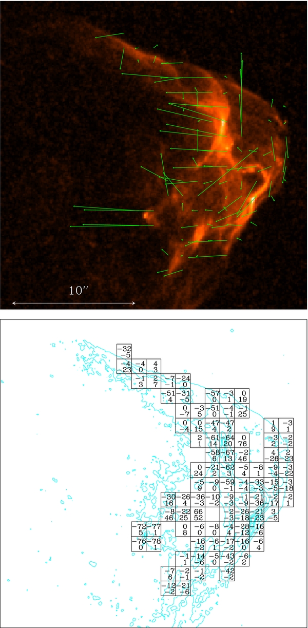
Figure 5. Relative Hα proper-motion map of HH 34S (see the description in Section 3.2). Top frame: the arrows show the proper motions (relative to the motion of HH 34S) computed in 24 square boxes. Bottom frame: the central regions of the cross-correlation boxes are shown, and within each of the boxes are written the components of the proper-motion velocities along (top number) and across (bottom number) the outflow axis.
Download figure:
Standard image High-resolution image3.3. Parameters Deduced from the HH 34 Kinematics
From the [S ii] kinematical map shown in Figure 3, we determine that the maximum velocity away from the outflow axis is v⊥ = 55 km s−1. The maximum relative velocity along the outflow axis is v|| = 87 km s−1 (along the extended outflow wing on the top of Figure 3).
With these values, we can then apply the relations deduced from a kinematical bow shock model by Raga et al. (1997), which can be written as

where vbs is the velocity with which the bow shock travels with respect to the surrounding medium, and ϕ is the angle between the outflow axis and the plane of the sky. With the values of v⊥ and v|| given above, from Equation (1) we then obtain vbs = 110 km s−1 and ϕ = 38°. Additionally, the measured proper motions imply that the environment into which HH 34S is travelling is moving away from the outflow source at a velocity ve = vT, 34S − v|| = 121 km s−1.
4. THE HH 34 JET
4.1. [S ii] Proper Motions
For calculating the proper motions for the chain of aligned knots within ∼30'' from the outflow source we restrict ourselves to the [S ii] frames, since the knots are considerably fainter in Hα, and the kinematics deduced from the [S ii] and Hα images do not differ significantly (see Reipurth et al. 2002).
The region with the knots within ∼30'' from the outflow source is shown in Figure 6. We see that within x < 11'' (7 × 1016 cm at 414 pc) from the source there are clear, marginally resolved emission peaks, and that for x > 11'' the knots are much more extended. Because of this qualitative difference, we have computed the proper motions in different ways.
- 1.Knots with x < 11''. We have carried out paraboloidal fits to the emission peaks of the successive knots, and then computed proper motions from the difference in knot positions. The identification chosen for the corresponding knots in the two time frames is given in the bottom frame of Figure 6.
- 2.Knots with x > 11''. We have defined boxes including the emission from the successive knots in the 1998.71 image (top frame of Figure 6), and boxes with the same size but with a displacement of 6 pixels (06) along the outflow axis in the 2007.83 image. The proper motion of these knots was determined from a paraboloidal fit to the peak of the cross-correlation function of the emission within the pairs of (displaced) boxes.

Figure 6. Top pair: the HH 34 jet in the 1998.71 (top) and 2007.83 (bottom) [S ii] images. Bottom pair: zoom of the region close to the source of the two frames. The emission peak on the left of the chain of knots corresponds to the position of the outflow source. The top two frames show the (shifted) boxes used to compute the cross-correlations of the knots at larger distances from the source. The crosses in the two bottom frames show the positions determined from direct paraboloidal fits to the emission peaks of the knots closer to the source. The yellow arrows (two bottom frames) show the assumed identifications of corresponding knot pairs in the two epochs.
Download figure:
Standard image High-resolution imageThe resulting proper motions are given in Table 1.
Table 1. [S ii] Proper Motions of the HH 34 Jet Knots
| Knota | xb | yb | vxc | vyc | tdynd |
|---|---|---|---|---|---|
| (1016 cm) | (1016 cm) | (km s−1) | (km s−1) | (yr) | |
| 1 | 0.80 | −0.03 | 171 | −2 | 15 |
| 2 | 1.24 | −0.05 | 202 | −8 | 20 |
| 3 | 2.22 | −0.17 | 171 | −9 | 42 |
| 4 | 2.90 | −0.26 | 175 | −20 | 53 |
| 5 | 3.86 | −0.30 | 164 | −4 | 75 |
| 6 | 4.94 | −0.17 | 163 | −9 | 96 |
| 7 | 5.59 | −0.20 | 141 | −3 | 126 |
| 8 | 6.04 | −0.18 | 162 | 0 | 119 |
| 9 | 6.49 | −0.25 | 165 | −5 | 125 |
| 10 | 8.09 | −0.18 | 156 | −5 | 166 |
| 11 | 8.47 | −0.23 | 156 | −5 | 173 |
| 12 | 9.55 | −0.33 | 142 | −3 | 214 |
| 13 | 10.89 | 0.05 | 148 | −3 | 234 |
| 14 | 11.49 | −0.14 | 148 | −3 | 247 |
| 15 | 12.50 | −0.18 | 148 | −13 | 268 |
| 16 | 13.64 | −0.24 | 138 | −9 | 313 |
| 17 | 15.06 | −0.21 | 133 | −17 | 359 |
| 18 | 17.54 | −0.33 | 143 | −1 | 390 |
Notes.
aThe successive knots away from the source are numbered consecutively.
bx and y are the offsets from the position of the source measured along and across the outflow axis in the 2007.83 frame. The angular separations have been converted into cm assuming a 414 pc distance to HH 34.
cVelocities along and across the outflow axis assuming a 414 pc distance.
dDynamical time computed as  .
.
Download table as: ASCIITypeset image
For the x > 11'' knots, we have also carried out paraboloidal fits to the emission peaks in the 2007.83 image. The offsets x (along the outflow axis) and y (perpendicular to the outflow axis) from the source position in the 2007.83 frame are given in Table 1 (for all of the knots). Two of the boxes defined for the x > 11'' knots actually contain two emission peaks (see Figure 6). For these boxes, in Table 1 we have made pairs of entries (entries 10/11 and 13/14) which share the same values of vx and vy (obtained from the cross-correlation within the box that includes the two peaks) but different x and y values (obtained from the fits to the peaks in the 2007.83 frame).
The top frame of Figure 7 shows the total plane-of-the-sky velocity  as a function of the position x of the knots, showing a general trend of decreasing vT for increasing distances from the source. It is clear that two knots show peculiar deviations from the general trend.
- 1.The second knot (knot 2 of Table 1) has vT ≈ 250 km s−1, approximately 40 km s−1 higher than the velocities of all of the other knots.
- 2.The seventh knot (knot 7 of Table 1) has a velocity vT ≈ 170 km s−1, about 30 km s−1 lower than the motions of its neighbors.

Figure 7. Top to bottom: proper-motion velocity vT, orientation angle α of the knots, orientation αv of the proper motions (see Figure 8), and dynamical time tdyn as a function of distance x from the outflow source for the knots along the HH 34 jet (see Sections 4.1 and 4.2).
Download figure:
Standard image High-resolution imageReipurth et al. (2002) obtained anomalously large motions for the knots closer to the HH 34 source. The fact that we are obtaining an apparently similar effect probably indicates that in this region there are strong changes in the morphologies of the knots, which result in large proper motions that do not represent the physical motion of the gas within the jet.
It is also not completely surprising that knot 7 (see Table 1) has a velocity lower than its neighboring knots. As can be seen in the two bottom frames of Figure 6, knot 7 shows an axially extended structure. This structure has an emission peak close to its leading edge in the 1998.71 frame, which partially disappears in the 2007.83 frame. This morphological change of course results in a lower value for the measured proper motion. For this knot, we have also computed proper motions using the cross-correlation function method (see above), and basically the same results (as with the peak emission fitting) are obtained.
From Table 1 we see that the values of vx are 1–2 orders of magnitude larger than the vy values for the corresponding knots. This result indicates that the proper motions are well aligned with the outflow axis. In order to quantify this, we define two angles:

where the angles α (between the source–knot direction and the outflow axis) and αv (between the proper-motion vector and the outflow axis) are defined in the schematic diagram shown in Figure 8. It is clear that for knots with time-independent morphology moving in ballistic trajectories, one will have α = αv.

Figure 8. Schematic diagram showing the definition of the orientation angle α of the knot position, and the orientation αv of the proper motion. It is evident that for ballistic motions we have α = αv.
Download figure:
Standard image High-resolution imageIn Figure 7, we show the values of α and αv (see Equation (2)) as a function of x computed from the knot positions and proper motions shown in Table 1. In the x ∼ 3 × 1016 cm region, there is a lateral excursion of the jet beam (reaching values of α ≈ −5°), which can be clearly seen in the bottom image of Figure 6. This excursion to larger deviations from the outflow axis can also be seen in the orientation angle αv of the proper motions. A comparison between the second and third panels of Figure 7 shows that in the x < 1.2 × 1017 cm region we have α ≈ αv to within the measurement errors, indicating that the motions are consistent with a ballistic motion of knots ejected with an ejection direction (on the plane of the sky) that changes by up to ∼5°.
For x > 1.2 × 1017 cm we have a different situation, with low values of α as a function of x, and with αv having an excursion to larger negative values (of up to ∼ − 7°). This result can be interpreted in two ways.
- 1.The knot motions in this region have measurable deviations from ballistic trajectories.
- 2.The spatially resolved knots in this region develop systematic side-to-side asymmetries which result in larger measured values for vy.
4.2. The Dynamical Time
With the values of the proper-motion velocities and the distance from the source, we can compute a dynamical time
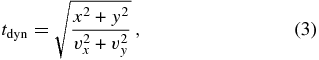
for each of the knots along the jet. The values of tdyn as a function of x are shown in the bottom frame of Figure 7 (also see the last column of Table 1).
We obtain an almost monotonically increasing tdyn versus x dependence, which indicates that the motions of the knots do not deviate substantially from ballistic motions. The only exception is knot 7 (indicated by an arrow in the bottom frame of Figure 7), which has a value of tdyn marginally higher than the dynamical times of knots 8 and 9 (see Table 1). This is again an indication that the measured proper motion of knot 7 might not correspond to the motion of the gas within this knot (see the discussion in Section 4.1).
4.3. Orientation with Respect to the Plane of the Sky
In order to determine the spatial velocity of the knots, it is of course necessary to determine the orientation angle of the outflow axis with respect to the plane of the sky. To this effect, we combine the tangential velocity vT (determined in Section 4.1) with radial velocities (with respect to the velocity of the local CO emission) for the HH 34 jet knots.
In Figure 9, we show the absolute values of the radial velocities determined by García López et al. (2008) from the [Fe ii] 1.64 μm emission of the HH 34 jet and counterjet. Given the remarkable jet/counterjet knot-to-knot symmetry seen in Spitzer images of the HH 34 outflow (Raga et al. 2011b), we would expect the jet and the counterjet to have very similar radial velocity versus position signatures.
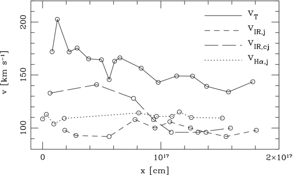
Figure 9. Proper-motion velocity (solid line), and radial velocities from Hα (dotted line; Beck et al. 2007), and [Fe ii] 1.64 μm (short dashes) lines for the HH 34 jet. The [Fe ii] 1.64 μm (García López et al. 2008) radial velocities of the HH 34 counterjet are also shown (long dashes). All of the velocities are plotted as a function of distance from the source.
Download figure:
Standard image High-resolution imageAlso shown in Figure 9 is the Hα radial velocity versus the position obtained for the high-velocity component of this line as a function of position (obtained by integrating the emission of the successive knots within a 1'' diameter diaphragm) from the two-dimensional spectra of Beck et al. (2007). These Hα velocities show a reasonably good agreement with the [Fe ii] 1.64 μm HH 34 jet radial velocities, but unfortunately the data of Beck et al. (2007) do not cover the x ∼ 2–8 × 1017 cm region (see Figure 9).
As can be seen in Figure 9, the [Fe ii] 1.64 μm jet/counterjet radial velocities agree well for the knots with x > 7 × 1016 cm, but show differences of up to ∼50 km s−1 for the knots closer to the outflow source. Possible interpretations for this discrepancy in the jet/counterjet radial velocities are as follows.
- 1.The jet and the counterjet have different orientations with respect to the plane of the sky. This could easily be obtained if this outflow is ejected from a source in orbital motion around a binary companion, resulting in a mirror symmetric jet/counterjet spiral structure (such as appears to be observed in the HH 111 outflow; see Noriega-Crespo et al. 2011).
- 2.The observed line profiles could have a contribution from jet emission scattered on dust present in the surrounding environment. A stronger scattered component in the counterjet could be responsible for the difference in the jet/counterjet radial velocities (such effects have been studied, e.g., by Feldman & Raga 1991, Calvet et al. 1992, and Henney 1994). Such a jet/counterjet asymmetry in the dust scattering might be expected because of the orientation (with respect to the plane of the sky) of a flattened, scattering structure perpendicular to the outflow axis.
Let us explore further the first of these possibilities. If we consider the jet/counterjet [Fe ii] 1.64 μm radial velocities at x ≈ 5 × 1016 cm (see Figure 9), using the corresponding proper-motion velocities of the knots along the jet, we would deduce ϕj ≈ 29° and ϕcj ≈ 40° orientation angles between the plane of the sky and the jet/counterjet (respectively). If we consider the radial velocities at x ≈ 1.4 × 1017 cm (in which the absolute values of the jet and counterjet radial velocities coincide), we obtain an orientation angle (with respect to the plane of the sky) of ϕ = 34° for both the jet and the counterjet.
From this, we would conclude that at x = 1.4 × 1017 cm, the jet and the counterjet lie along an axis with a ϕ = 34° orientation with respect to the plane of the sky, and that closer to the source (at x ≈ 5 × 1017 cm) the jet and counterjet have mirror symmetric deviations (along the line of sight) of ∼5°–6° from this axis. As can be seen in Figure 7 (in the α versus x plot), the jet shows plane-of-the-sky deviations from the average outflow axis of ∼5°, although the maximum deviations occur at x ≈ 3 × 1016 cm.
4.4. Ejection Velocity versus Time
Assuming ballistic motions for the knots, we can then calculate the past ejection velocity vj as a function of ejection time t = −tdyn (t = 0 corresponding to 2007.83; see Equation (3)). We calculate the velocity at which each of the knots was ejected in two ways.
- 1.vj = vT/cos 35°; in other words, we take the proper-motion velocity
 and assume that all of the knots move at a ϕ = 35° angle with respect to the plane of the sky.
 - 2., where vr is the [Fe ii] 1.64 μm radial velocity measured by García López et al. (2008) for the HH 34 jet knots. To do this, we take the positions at which the radial velocities were measured, and choose the proper motion of the optical knot closest to each of these positions.
The results of this exercise are shown in Figure 10 (where, following the discussion of Sections 4.1 and 4.2, we have eliminated knots 1, 2, and 7). It is clear that the ejection velocity time histories computed in the ways described above both give a general trend of increasing velocities from ∼400 yr ago to the present time.
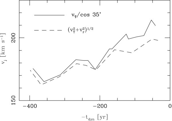
Figure 10. Reconstructed ejection velocity time history. The solid line is calculated assuming a position-independent angle of 35° between the outflow axis and the plane of the sky. The dashed line is calculated considering our proper motions (see Table 1) and the Fe ii] 1.64 μm of the HH 34 jet of García López et al. (2008).
Download figure:
Standard image High-resolution image4.5. Ballistic Trajectory Plot
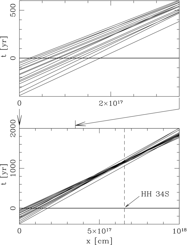
If we take the proper-motion velocities vT, k, and assume that the knots move ballistically, the plane-of-the-sky position xk(t) of an arbitrary knot k has a time dependence of the form

where xk, 0 is the 2007.83 position of knot k (the measured values of xk, 0 and vT, k are given in Table 1).
Figure 11 shows the trajectories in the (x, t)-plane given by Equation (4) for the HH 34 jet knots. In the two frames of this figure, the 2007.83 positions of the knots correspond to the intersection of the knot trajectories with the x-axis. We show the trajectories for all of the measured knots (see Table 1) except knots 1, 2, and 7 (see Sections 4.1 and 4.2).
Figure 11. Ballistic trajectories in the (x, t) (position–velocity) plane calculate from the observed proper motions. The two frames show the same trajectories, but cover different extents of the (x, t) plane. The present-day position (t = 0) of HH 34S is indicated in the bottom frame.
Download figure:
Standard image High-resolution image
In the top frame of Figure 11, we see that the fact that the successive knots do not have identical velocities results in trajectory crossings (i.e., in collisions between successive knots, given the fact that the motions are quite well aligned). The first trajectory crossings will occur at t ∼ 200 yr and at a distance of ∼2 × 1017 cm away from the source, down the HH 34 outflow axis.
The bottom frame of Figure 11 shows a more extended time evolution of the knot positions. This plot shows that the knot trajectories have a remarkable convergence at the point (xc, tc) ≈ (5 × 1017cm, 900 yr). This is a direct indication that at this position and time the knots will merge in order to form a major mass concentration.
As shown in the bottom frame of Figure 11, the region of convergence of the knot trajectories lies ∼1016 cm upstream of the present-day position of HH 34S. Therefore, we conclude that in the proper motions of the knots along the HH 34 jet we see direct evidence for the formation of a massive structure (possibly resembling the present-day HH 34S) some ∼900 yr in the future.
5. SUMMARY AND CONCLUSIONS
With archival [S ii] 6716+30 and Hα HST images of HH 34 with a ∼9 yr time base, we have carried out proper-motion measurements of the HH 34S bow shock and of the aligned knots within ∼30'' from the outflow source (for these knots, only the [S ii] images were analyzed). Even though these images have been published before (Reipurth et al. 2002 and Hartigan et al. 2011), they have not yet been combined to carry out quantitative proper-motion measurements.
For the HH 34S bow shock we first determined the average proper motion (through a cross-correlation of the emitting structure), and then shifted the images of one of the two epochs with this measured displacement. We then carried out cross-correlations in a grid of 24 square boxes, and determined the motion of the emitting structures (within the boxes) by fitting the peak of the cross-correlations. In this way we constructed [S ii] and Hα "relative motion map" (Figures 3 and 5) that show trailing motions along the bow shock wings and expansion motions in the head of the bow shock. An interpretation of these effects has been discussed by Raga et al. (2002).
We have also determined the [S ii] proper motions of the aligned knots along the HH 34 jet. We obtain a number of interesting results.
- 1.The knots have velocities in the 135–200 km s−1 range. These velocities agree to within ∼10%–20% with the [S ii] proper motions of Reipurth et al. (2002), after correcting for the fact that these authors used a distance of 460 pc to HH 34 (the 414 pc distance suggested by Menten et al. 2007 has been used in our paper).
- 2.
- 3.We find that the dynamical time tdyn = x/vT (where x is the distance from the source and vT is the proper-motion velocity of one of the knots) is a monotonically increasing function of x. This indicates that the motion of the knots is closely ballistic.
- 4.Considering radial velocity measurements from the literature, we see that the HH 34 jet might also have a ∼5° deviation along the line of sight. The jet/counterjet [Fe ii] 1.64 μm radial velocity asymmetry found by García López et al. (2008) indicates the possible presence of mirror symmetric deviations from the average outflow axis, which might be a result of an orbital motion (around a binary companion) of the outflow source (see Figure 9).
- 5.Considering ballistic motions for the knots, it is possible to reconstruct the ejection velocity time variability over the past ∼400 yr. This exercise gives an ejection velocity with a systematic increase over this time period (Figure 10).
- 6.If one draws the ballistic trajectories (corresponding to the present-day, plane-of-the-sky positions and velocities) of the HH 34 knots, one finds that only a few knot collisions will occur in the future ∼300 yr. On the other hand, in ∼900 yr most of the HH 34 jet knots that we observe today will merge (see Figure 11). This merger will occur at ∼5 × 1017 cm (∼80'') away from the outflow source. It is not unlikely that this structure could evolve to resemble the present-day HH 34S bow shock (at ∼100'' from the source).
In this way, the proper-motion velocities of the HH 34 jet knots within ∼30'' from the source provide direct evidence of the future formation of a large mass concentration, possibly resembling the present-day HH 34S bow shock. The only requirement for obtaining this prediction is that the knots should move in approximately ballistic trajectories. As ballistic motions are also directly implied by the observations (see Section 4.2 item 3 above), the future formation of a large mass concentration appears to be inevitable.
For deriving this result, we have of course assumed that the emission along HH 34 traces the positions of physical "knots." This situation is obtained in variable ejection jet models (e.g., Raga et al. 1990; Cantó et al. 2000), which produce "internal working surfaces" into which the ejected material is rapidly piled up, and which then move away from the source as quasi-ballistic, constant velocity clumps. These knots have a leading bow shock and an internal "jet shock" which produce the observed emission. The emission behind the "jet shock," the head of the bow shock, and the bow shock structure as a whole share the motion of the clump (even though small-scale inhomogeneities along the bow shock wings slip backward with respect to the clump motion; see Raga et al. 1988, 1997). There is now little doubt that the knots along the HH 34 jet are indeed knots produced by an ejection variability, since a counterjet with surprising knot-to-knot symmetry has been recently discovered (see García López et al. 2008; Raga et al. 2011b).
There is the possibility that the material ejected from the HH 34 outflow source could be slowed down as a result of the entrainment of low-velocity, ambient material. Such an effect could in principle produce a "deceleration" such as the one that we are observing along the HH 34 knot chain (which we are interpreting above as evidence for a decreasing ejection velocity as a function of time). However, this is unlikely to be the case, since numerical simulations of well-aligned, variable jets do not show such an effect, as the leading bow shock mostly clears out the surrounding environment, and the following knots travel within a low-density cocoon. For example, the variable jet simulations of Völker et al. (1999) and Masciadri et al. (2002b) show that (following an initial acceleration over distances similar to the separation between knots) the "internal working surfaces" that result from an ejection velocity variability have constant velocity, ballistic motions.
Interestingly, the bow shocks observed along the "HH 34 giant jet" (at distances beyond HH 34S and HH 34N, extending out to ∼1.5 pc from the outflow source; see Bally & Devine 1994) show a systematic trend of decreasing velocities versus distance, which cannot be interpreted straightforwardly as the result of a decreasing ejection velocity as a function of time (Cabrit & Raga 2000), and therefore has to be a result of braking due to interaction with the environment (as suggested by Devine et al. 1997). Simulations of the HH 34 giant jet do show this effect (Masciadri et al. 2002a), which is present due to the fact that a precession of the outflow axis exposes the successive working surfaces to direct interaction with the surrounding environment. Such an effect would not be expected along the chain of knots close to the HH 34 outflow source (at <30''), for which the precession of the outflow axis produces only a small misalignment. Therefore, the observed "deceleration" along this chain of knots is indeed evidence for an ejection velocity that has decreased as a function of time over the past ∼400 yr.
This paper is based on observations made with the NASA/ESA Hubble Space Telescope, and information obtained from the Hubble Legacy Archive, which is a collaboration between the Space Telescope Science Institute (STScI/NASA), the Space Telescope European Coordinating Facility (ST-ECF/ESA), and the Canadian Astronomy Data Centre (CADC/NRC/CSA). The work of A.R., A.R.G., and V.L. was supported by the CONACyT grants 61547, 101356, and 101975. We thank John Bally (the referee) for helpful comments which led to the inclusion of Figure 6 and to the discussion at the end of Section 5.