


ABSTRACT
We study the thermal evolution of super-Earths with a one-dimensional (1D) parameterized convection model that has been adopted to account for a strong pressure dependence of the viscosity. A comparison with a 2D spherical convection model shows that the derived parameterization satisfactorily represents the main characteristics of the thermal evolution of massive rocky planets. We find that the pressure dependence of the viscosity strongly influences the thermal evolution of super-Earths—resulting in a highly sluggish convection regime in the lower mantles of those planets. Depending on the effective activation volume and for cooler initial conditions, we observe with growing planetary mass even the formation of a conductive lid above the core-mantle boundary (CMB), a so-called CMB-lid. For initially molten planets our results suggest no CMB-lids but instead a hot lower mantle and core as well as sluggish lower mantle convection. This implies that the initial interior temperatures, especially in the lower mantle, become crucial for the thermal evolution—the thermostat effect suggested to regulate the interior temperatures in terrestrial planets does not work for massive planets if the viscosity is strongly pressure dependent. The sluggish convection and the potential formation of the CMB-lid reduce the convective vigor throughout the mantle, thereby affecting convective stresses, lithospheric thicknesses, and heat fluxes. The pressure dependence of the viscosity may therefore also strongly affect the propensity of plate tectonics, volcanic activity, and the generation of a magnetic field of super-Earths.
Export citation and abstract BibTeX RIS
1. INTRODUCTION
The recent discovery of super-Earths (e.g., Borucki et al. 2011; Queloz et al. 2009) has increased the interest to better understand such planets. Super-Earths are extrasolar rocky planets that are 1–10 times more massive than the Earth but with radii between one and two Earth radii, allowing for a composition of mainly iron and silicates. The thermal evolution, the tectonic style but also the potential habitability of super-Earths have been studied but are controversial. In particular, the likelihood of these planets having plate tectonics (hereafter PT) or a magnetic field is under debate (e.g., for PT: Korenaga 2010; O'Neill & Lenardic 2007; Stein et al. 2011; Valencia et al. 2007; Van Heck & Tackley 2011; e.g., for magnetic fields: Driscoll & Olson 2011; Gaidos et al. 2010; Tachinami et al. 2011).
So far these models primarily neglect pressure effects, especially on the viscosity, and assume an entirely convecting mantle (Gaidos et al. 2010; Korenaga 2010; Kite et al. 2009; O'Neill & Lenardic 2007; Sotin et al. 2007; Valencia et al. 2006; Van den Berg et al. 2010; Van Heck & Tackley 2011). The assumption that pressure effects are negligible for super-Earths seems, however, questionable: already for Earth conditions, where the mantle pressure reaches 135 GPa, the viscosity (Mitrovica & Forte 2004) and the thermal conductivity (Hofmeister 1999) are crucially affected by pressure. For a 10 Earth mass super-Earth, the mantle pressure increases above 1 TPa (Valencia et al. 2006; see our Figure 1), and hence pressure effects might be even more important than they are for the Earth.
Figure 1. Key data for differentiated super-Earths with an iron-rich core and a silicate mantle. The table shows the approximate core-mantle boundary pressures Pcmb, planetary and core radii (Rp and Rc), and average mantle and core densities (ρm and ρc) for three different planet masses M relative to the Earth mass MEarth (derived in Section 2 with the mass-radius scalings from Valencia et al. 2006). Download figure:

Recent studies (Karato 2011; Stamenković et al. 2011) have highlighted the importance of pressure effects on the thermal and transport properties of mantle rock and the implications for super-Earth rheologies. Karato (2011) and Stamenković et al. (2011) differ in their conclusion about the pressure dependence of mantle viscosity for super-Earths: Karato (2011) suggests an almost isoviscous mantle for super-Earths assuming interior temperatures as discussed in the literature (e.g., Papuc & Davies 2008; Sotin et al. 2007; Valencia et al. 2006) and hence supports the idea of the entirely convecting mantle.
Contrary to this study, Stamenković et al. (2011) find a strongly increasing viscosity along the same thermal profiles, as well as increasing thermal conductivities, and a decreasing thermal expansivity for more massive planets. The authors speculate that this could lead to a highly sluggish convection and the formation of stagnant zones above the core-mantle boundary (CMB) of such planets, termed CMB-lids. This reduction of convective vigor could have a profound impact on the thermal evolution, magnetic field generation, and possibly PT.
The discrepancy between Karato (2011) and Stamenković et al. (2011) reflects the present lack of knowledge of the properties of mantle rock at high pressure. But it also motivates the study of the thermal evolution of super-Earths for a variety of rheologies to obtain a more complete picture of what could actually be happening inside rocky exoplanets.
In the present paper, we model the interior thermal evolution of super-Earths with a pressure- and temperature-dependent mantle viscosity, and compare it to the thermal evolution of a planet with a purely temperature-dependent mantle viscosity. We develop a parameterized one-dimensional (1D) convection model that self-consistently considers a potential CMB-lid. We also compare the results of the parameterized model with those of a 2D spherical convection model to test the chosen 1D approximation.
The advantage of parameterized models is their ability to study the thermal evolution of planets using parameter values relevant for super-Earths—which is not yet possible with 2D convection models. The focus of this paper is to apply the parameterized model to a large parameter space and further discuss the importance of initial conditions, the effects of PT and compressibility, and implications for the propensity of PT and magnetic field generation of super-Earths.
The paper is organized as follows. First, we describe the planetary model including scalings for the planetary radius, average mantle density, and the temperature- and pressure-dependent mantle viscosity with increasing mass for super-Earths (Section 2). In Section 3, we present the 1D parameterized thermal evolution model for planets in the stagnant lid (SL) regime, i.e., one-plate planets, which is based on boundary layer stability analysis. The model is later modified to as well include planets in a PT regime. We introduce the parameters used (Section 4) to then present the results of the 1D model for SL as well as PT planets in Section 5. In Section 6, we compare our 1D model with a 2D convection model, discuss among others the limitations of the 1D model, the effect of compressibility on the thermal evolution, and elaborate on the propensity of PT and dynamo generation in case of a temperature- and pressure-dependent viscosity.
2. THE PLANETARY MODEL
For the planetary model we use the mass-radius scaling from Valencia et al. (2006). Our scaling parameter is the planetary mass to Earth mass ratio M = Mp · (MEarth)−1 ranging from 1 to 10. The core mass fraction ( fc) is assumed to correspond to the Earth ratio of fc ∼ 0.326. Then the planetary radius for super-Earths Rp scales with the average Earth radius REarthp as

This relation does not vary significantly for mantle compositions with various MgO, MgSiO3, or iron ratios (e.g., Valencia et al. 2006). Due to the assumption of a constant fc Valencia et al. (2006) find that the core radius Rc scales with the average Earth core radius REarthc approximately as

and the average mantle density is hence given by

The average core density is defined by

The surface gravity g0(M) scales with the universal gravitational constant G = 6.673 × 10⁻¹¹ m3 kg−1 s−2 or the surface gravity of Earth gEarth0 with

g(M, P) is almost constant throughout the mantle of each planet (Wagner et al. 2011) and we set g(M, P) = g0(M).
The composition of the mantles of super-Earths and thus the amount of radioactive heat sources is not known. We assume a standard depleted mantle composition following McDonough & Sun (1995), which contains radiogenic heat sources equivalent to a radiogenically produced Earth heat flux of about 20 TW today (i.e., QEarthm(t = 4.5 Gyr) = 2.3 × 10⁻⁸ W m−3 for present Earth)

Qm is the volumetric density of radiogenic heat sources (W m−3) homogeneously distributed in the mantle and decaying with time t, corresponding to the time after the planet's formation. Each radiogenic species is characterized by its half-life τ1/2, j and heat generation rate in Q*j in (W kg−1), which are summarized in Table 4. We further assume that there are no radiogenic heat sources in the core, although it has been suggested that the likelihood of an incorporation of radiogenic elements into the core increases with pressure (e.g., Gessmann & Wood 2002).
As discussed above, the mantle rheology of super-Earths is not known and currently debated (Karato 2011; Stamenković et al. 2011). The creep behavior is expected to be primarily controlled by (Mg, Fe)SiO3 post-perovskite and (Mg, Fe)O ferropericlase. Hot (i.e., with lower mantle temperature above ∼10,000 K) super-Earths might be additionally affected by cotunnite- or Fe2P-type SiO2 (Umemoto et al. 2006; Tsuchiya & Tsuchiya 2011). However, we focus on the general influence of a pressure- and temperature-dependent viscosity in the mantle; thus, details concerning the viscosity law are not relevant in this study. We assume a Newtonian rheology (analogous to Karato 2011 and Stamenković et al. 2011), which leads approximately to a pressure- and temperature-dependent Arrhenius-type dynamic viscosity η(P, T):
where Rg ≈ 8.3145 J mol−1 K−1 is the universal gas constant, P is the pressure, T is the temperature, b is a constant, E* is the activation energy describing the temperature-viscosity coupling, and V*eff(P) is the effective activation volume describing the pressure-viscosity coupling (for details, see Stamenković et al. 2011). For V*eff(P) = 0 we have a purely temperature-dependent viscosity. V*eff(P) is thought to decrease with pressure (Poirier 1985), although Karato (2008) speculates that it might even remain constant. We neglect for simplicity the pressure dependence of the effective activation volume to study the general differences between pressure-dependent and pressure-independent viscosity models and assume instead for each planet a characteristic, constant effective activation volume throughout the mantle V*eff(M) = constant (for parameter values see Section 4).
For a better comparison between the models, we introduce a reference viscosity ηref = η(Pref, Tref) at reference pressure Pref and reference temperature Tref. In that case, the viscosity is given by
The effect on the dynamics and the thermal evolution caused by the variation in viscosity throughout the mantle of the studied planets is assumed to be larger than the effects due to a depth variation of the other thermal properties influencing convection, such as the mantle thermal expansivity αm (K−1), or the mantle thermal conductivity km (W m−1 K−1) (Stamenković et al. 2011). Thus, at first we keep αm and km constant and use instead average Earth mantle reference values similar to Papuc & Davies (2008), Valencia et al. (2007), and Valencia & O'Connell (2009).
The pressure scales approximately with the average mantle density according to P(R) ≈ ρm · g · (Rp − R) for a radius R. To remain consistent with the definition of the pressure via the average mantle density we use for all scalings the average mantle density (Equation (3)) analogous to Papuc & Davies (2008), Valencia et al. (2007), and Valencia & O'Connell (2009). The thermal mantle diffusivity κm(m2 s−1) is then calculated accordingly with κm = km(ρmCm)−1, where Cm (J kg−1 K−1) is the mantle specific heat at constant pressure, which is approximately constant for all studied planets (Stamenković et al. 2011). All used parameters are defined in Section 4.
3. 1D PARAMETERIZED CONVECTION MODEL
Parameterized convection models have been widely used to calculate the thermal evolution of terrestrial planets (e.g., Grott & Breuer 2008; Schubert et al. 2001; Stevenson et al. 1983). These models are based on a stability analysis of boundary layers that have been derived for either isoviscous cases or for cases with temperature-dependent viscosities where V*eff = 0 (e.g., Schubert et al. 2001).
As we want to study pressure-dependent rheologies, we need to modify existing 1D models in particular to account for the potential presence of a sluggish or stagnant layer, a CMB-lid (Lc), above the CMB. Based on linear stability analysis we develop a parameterized 1D convection model, including pressure dependence of the viscosity and demand a smooth convergence into a classical 1D local boundary layer model for V*eff = 0 as described by, e.g., Schubert et al. (2001).
The convecting mantle consists of an adiabatic zone between the radii Rm and Rb and two boundary layers (δu, δc) (see Figure 2). This convective zone is embedded by an SL (with thickness L) on top and in some cases by a CMB-lid (with thickness Lc) above the planet's core, depending on rheology and interior temperatures.
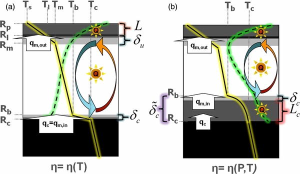
Figure 2. Depth profile of temperature (solid line) and viscosity (dashed line) for two viscosity cases: (a) a purely temperature-dependent viscosity (V*eff = 0); here, a thin lower thermal boundary layer δc (light gray) is above the CMB. The heat flux into the mantle equals the heat flux out of the core qc = qm,in; and (b) a strongly pressure-dependent as well as temperature-dependent viscosity. Here a thick thermal conductive zone  is located above the CMB, consisting of a stagnant CMB-lid Lc (dark gray) and a lower thermal boundary layer δc (light gray). The heat flux into the convective mantle is qm,in ≠ qc. The difference between qm,in and qc is due to heating by radiogenic heat sources in the conductive zone
  . The decaying radiogenic heat sources are represented by Q. The temperature profile from Rm in the upper mantle to Rb is adiabatic, and lies below an upper thermal boundary layer (light gray) and an upper stagnant lid (dark gray). Note that in the case of plate tectonics there is no upper stagnant lid and Rl = Rp and Tl = Ts (Section 5.2). We assume (analogous to Gaidos et al. 2010) an adiabatic temperature distribution in the core (black region).
Download figure:
Standard image High-resolution imageThe thermal boundary layers (δu, δc) are part of the convective system and are modeled as conductive zones of thermal instabilities, which are assumed to drive the convection (e.g., Turcotte & Schubert 2002). They grow on short geological timescales (e.g., Turcotte & Schubert 2002, p. 273) until they become unstable and rise or fall as hot or cold plumes, respectively. The thickness of each boundary layer δ = (δu, δc) is given by (e.g., Stevenson et al. 1983)

where ηδ is the characteristic viscosity (see Sections 3.1 and 3.2) of the thermal boundary layer, ΔTδ is the temperature jump across the boundary layer, and Ra(δ) is the characteristic Rayleigh number of the boundary layer.
Stability analysis assumes that the characteristic Rayleigh number of the boundary layers equals the critical Rayleigh number Racrit of these mantle sub-systems, which represents the Rayleigh number necessary to initiate convection in the boundary layer (e.g., Howard 1966). This method is commonly used in the literature (e.g., Fu et al. 2010; Schubert et al. 1979; Solomatov 1995; Stevenson et al. 1983; Valencia & O'Connell 2009).
The conductive heat flux through the boundary layer qδ is assumed to represent the energy flux streaming into or out of the convecting mantle
We define a lower mantle conductive zone  . When no CMB-lid exists, especially for V*eff = 0, this zone corresponds directly to the lower thermal boundary layer,
  . However, when pressure effects are strong enough this zone contains the lower thermal boundary layer δc and a CMB-lid Lc,
  .
.
The thermal evolution of a planet is modeled starting from an initial temperature profile corresponding to the time after core formation, and the evolution is determined by the energy balance equations for the core and the mantle assuming SL convection (e.g., Grott & Breuer 2008). We later show how active PT alters the thermal evolution.
The energy equations of the core and mantle are given by


where ρm and ρc are the average mantle and core densities, Cm and Cc are the average mantle and core specific heat capacities, and Vc = (4π/3)R3c and Ac = 4πR2c are the core volume and surface, respectively. The convective mantle volume is Vlb = (4π/3)(R3l − (Rb − δc)3), where Rl = Rp − L is the radius to the base of the SL, L is the SL thickness, and Rb is the radius at the top of  ; Al = 4πR2l and Ab = 4π(Rb − δc)2 are the corresponding surfaces.
〈T〉m and 〈T〉c are the average temperatures in the mantle and the core, respectively,
where R is radius, T(R) is the thermal profile through the planet's interior, and Tm and Tc are the upper mantle and CMB temperature, respectively (compare Figure 2). Here (εm, εc) are constants relating the average mantle and core temperatures to the upper mantle Tm and CMB temperature Tc, respectively. For the core we assume an adiabatic thermal profile similar to Gaidos et al. (2010). See Appendix A for the derivation of the thermal profile in the core.
To solve Equations (11) and (12), we have to define the heat fluxes in and out of the reservoirs, i.e., the core and the mantle, and to find a criterion that describes the lower mantle structure, i.e.,  , δc, and Lc. Although it is possible to define the boundary between the SL and the upper thermal boundary layer (see below), the separation of the CMB-lid Lc and the lower thermal boundary layer δc cannot yet be satisfactorily described—nonetheless, we later suggest a potential method and discuss the implications on our results. Thus, the convective mantle volume is underestimated and its lower surface area is overestimated in the energy equation of the mantle (Equation (12)) as they are approximated by Vlb = (4π/3)(R3l − (Rb − δc)3) ≈ (4π/3)(R3l − Rb3) and Ab = 4π(Rb − δc)2 ≈ 4πR2b; i.e., the lower mantle thermal boundary layer is neglected in the convective zone. Generally, the difference is expected to be small as the thermal boundary layer should be thin. However, we discuss cases for which the thickness of the lower thermal boundary layer δc can be large (see Section 6.2).
In the following, we define the scaling relationships for the upper and lower mantle separately. In the upper mantle pressure effects are minor and we can hence rely on classic boundary layer stability models (Schubert et al. 2001).
3.1. Upper Mantle
For mantle viscosity contrasts larger than ∼3–4 orders of magnitude a stagnant layer forms on top of the convecting mantle (e.g., Solomatov 1995). Typical viscosity contrasts in the silicate mantles of terrestrial planets can be on the order of many magnitudes due to the interior temperature distribution, placing these planets into the so-called SL regime. Just below the SL is the upper thermal boundary layer δu (Figure 2). The viscosity contrast across this upper thermal boundary layer has been shown to be small, i.e., a factor of ∼10 (Davaille & Jaupart 1993; Grasset & Parmentier 1998) and we follow the approach of Dumoulin et al. (2005) assuming that the critical Rayleigh number of the upper boundary layer Raucrit is approximately the critical Rayleigh number of an isoviscous system Raucrit ≈ Racritiso ≈ 500 (Dumoulin et al. 2005). In that case the corresponding Rayleigh number for the upper boundary layer is defined for the lowest viscosity of the layer η(Rm), which is at the base of δu at the radiusR = Rm(Pm, Tm).
This defines the upper thermal boundary layer as a function of the critical Rayleigh number for isoviscous convection, i.e., Ra(δu) = Raucrit ≈ Raisocrit for a temperature- and pressure-dependent viscosity η(P, T), compare Equation (9)

The heat flux out of the mantle qm,out is then defined as the conductive heat flux through the upper thermal boundary layer:

In the case of PT, we assume that Tl is equal to the surface temperature Ts (e.g., Breuer & Spohn 2003). In the case of SL convection, we need to specify the temperature Tl at the base of the SL. As stated above, the viscosity contrast through the upper thermal boundary layer is approximately one order of magnitude (note that this limitation in the viscosity contrast for the upper thermal boundary layer is not required when modeling PT). Hence, the temperature Tl defining the base of the SL can be calculated as a function of the upper mantle temperature Tm and the viscosity law (Equation (8)):
For a solely temperature-dependent viscosity and RgTmln 10 ≪ E*, Equation (17) can be transformed into
which excellently approximates the experimental results for Tl by, e.g., Davaille & Jaupart (1993). We then calculate the evolution of the lithospheric thickness L(t) via the energy balance at the base of the SL neglecting volcanic heat transfer (Schubert et al. 1979; Spohn 1991):

To solve this SL growth equation (Equation (19)) we need to determine the upper mantle temperature Tm(t) and the thermal gradient at the SL base  . The thermal gradient at the base of the SL can be calculated by integrating the time-independent heat conduction equation:
with the SL base temperature Tl and the surface temperature Ts imposing a determined boundary problem. Note that for simplicity we use the steady-state heat solution because the typical relaxation time in the lithosphere is of the order of τ = L2/κm ≈ 100 Myr. This is much smaller than the relaxation time of the mantle, which is of the order of a few Gyr.
3.2. Lower Mantle
To calculate the upper mantle temperature Tm(t) we need to determine the heat flux into the convecting mantle qm,in. For this we have to specify the lower mantle energy budget—here pressure effects are crucial and we suggest a parameterization that considers a potential stagnant zone in the lower mantle.
The heat fluxes out of the core qc and into the convective mantle qm, in are described via the thermal gradients at the top and the base of the total lower mantle conductive zone  , respectively (see Figure 2),


These heat fluxes can be determined from the conductive thermal profile in  . As the stagnant CMB-lid and
  can comprise a substantial part of the mantle, we have to consider the radiogenic heat sources Qm and the time-dependent heat equation:
To solve for Equations (21)–(23), we need to determine the thickness of  . The conductive lower mantle layer
  is assumed to be at the verge of convective stability. Thus, we can compute the thickness of
  similarly to the upper thermal boundary layer, by specifying the critical Rayleigh number Raccrit of
  based on a characteristic viscosity ηc and the temperature contrast |Tc − Tb| of this layer:

The critical Rayleigh number of such a layer depends on the viscosity contrast Δη through it. This has originally been derived for pressure-dependent viscosities, which increase with depth, by Schubert et al. (1969), and for solely temperature-dependent viscosities, which decrease with depth, by Stengel et al. (1982) (see as well, e.g., Dumoulin et al. 2005 and Solomatov 1995). Based on these findings, we approximate the critical Rayleigh number of a layer with a viscosity contrast Δη by

where Raisocrit ≈ 500 is the critical Rayleigh number for an isoviscous system and ϕ is a constant.
This equation holds when the Rayleigh number is defined for the lowest viscosity of the system and when the viscosity monotonically increases or decreases (Figure 3). The value of ϕ varies approximately between ∼10 and ∼60 depending on the boundary conditions, the viscosity law, and the amount of internal heating (e.g., Dumoulin et al. 2005; Schubert et al. 1969; Solomatov 1995; Turcotte & Schubert 2002). We choose for our calculations ϕ equal to 11.74 according to Dumoulin et al. (2005)—additional tests have shown that a variation in ϕ between 10 and 60 does not change our findings. The value ϕ · [ln (Δη)]4 corresponds to the asymptotic limit of the critical Rayleigh number for large viscosity contrasts, but is generally used for viscosity contrasts above ∼3–4 orders of magnitude (e.g., Solomatov 1995; Fu et al. 2010). We note that Fu et al. (2010) use for smaller viscosity contrasts of (Δη ⩽ 103)a critical Rayleigh number of ∼1000–2000 but define the reference Rayleigh number at the average viscosity of the system. Due to the larger reference viscosity for the Rayleigh number we find this approach to be approximately consistent with our method.
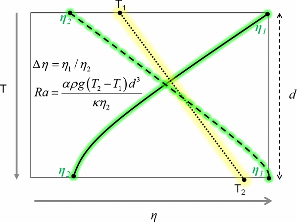
Figure 3. Layer of thickness d with a purely temperature-dependent viscosity decreasing (solid), a purely pressure-dependent viscosity (dashed) increasing, and the temperature (dotted) increasing with depth. We approximate the critical Rayleigh number of this system with Racrit(Δη) ≈ max {Raisocrit, ϕ · [ln (Δη)]4}. Racrit(Δη) depends on the viscosity contrast Δη and is defined for Rayleigh numbers at the lowest viscosity of the system (here η2) when the viscosity steadily increases or decreases with depth.
Download figure:
Standard image High-resolution imageWe can define the lower mantle conductive zone  using Equations (24) and (25), setting the critical Rayleigh number equal to Raccrit = Racrit(Δη) with Δη = max (η(Rc)/η(Rb), η(Rb)/η(Rc)) and the characteristic viscosity ηc = min {η(Rc), η(Rb)}:
For V*eff = 0 the minimal and hence characteristic viscosity is η(Rc) at the CMB (for illustration see Figures 2 and 3). In this case we find that, although the initial temperature contrast and thus the related viscosity contrast across  can be large, Δη quickly (<500 Myr) decreases below one order of magnitude due to the planet's efficient heat transport, resulting in Racrit ≈ Raisocrit and
  just as expected for a standard boundary layer model without pressure dependence. This simplifies for V*eff = 0 the lower mantle heat flux to
  .
.
When pressure effects lead to a viscosity increase through  with depth, as shown in Figure 2, our approach in determining
  is analogous to the determination of the upper conductive zone, consisting of the SL and the upper thermal boundary layer δu as suggested by Solomatov (1995). In this strongly pressure-dependent viscosity case, the minimal and therefore characteristic viscosity is η(Rb) at the top of
  .
.
4. PARAMETERS
In this section, fixed and varied input parameters are described and summarized in Tables 1–4. We compare the dynamics and thermal evolution of three planets with M = 1, 5, and 10, and calculate the thermal evolution for 13 Gyr, which is approximately the estimated age of the universe (Jarosik et al. 2011). As reference viscosity we use ηref = η(0, 1600 K) ≈ 1021 Pa, a typical viscosity for Earth's upper mantle (e.g., Mitrovica & Forte 2004; Turcotte & Schubert 2002, p. 273) and an activation energy of E* ≈ 300 kJ mol−1. These values are close to the results from Yamazaki & Karato (2001) for Earth mantle material, and are in agreement with the results of Stamenković et al. (2011) for rocky super-Earth mantles.
Table 1. Fixed Parameters Chosen for this Study
| Input Parameters | ||||
|---|---|---|---|---|
| Variable | Physical Meaning | Value | Units | Ref |
| Earth reference values | ||||
| MEarth | Earth mass | 5.974 × 1024 | kg | 1 |
| REarthp | Earth planetary radius | 6371 | km | 1 |
| REarthc | Earth core radius | 3480 | km | 1 |
| gEartho | Earth surface acceleration | ∼9.81 | ms−2 | 1 |
| Parameters for all planets | ||||
| Ts | Surface temperature | ∼290 | K | 1 |
| fc | Core mass fraction | 0.3259 | ... | 1 |
| km | Mantle thermal conductivity | 4 | Wm−1 K−1 | 2 |
| αm | Mantle thermal expansivity | 2 × 10⁻⁵ | K−1 | 2 |
| Cm | Mantle heat capacity at constant pressure | ∼1250 | Jkg−1 K−1 | 3 |
| Cc | Core heat capacity at constant pressure | ∼800 | Jkg−1 K−1 | 4 |
| E* | Activation energy | 300 | kJ mol−1 | 3 |
| ηref | Reference viscosity | 1021 | Pas | 3 |
| Tref | Reference temperature | 1600 | K | 3 |
| Pref | Reference pressure | 0 | Pa | 3 |
| ϕ | Critical Rayleigh number constant | 11.74 | ... | 5 |
References: (1) Turcotte & Schubert 2002; (2) Stevenson et al. 1983; (3) Stamenković et al. 2011; (4) Buffett et al. 1996; (5) Dumoulin et al. 2005.
Download table as: ASCIITypeset image
Table 2. Viscosity Models Used in this Study to Investigate Three Model Planets (M = 1, 5, 10), with the Effective Activation Volumes in (cm3 mol−1)
| Viscosity Models | ||||
|---|---|---|---|---|
| M (MEarth) | 1 | 5 | 10 | Model |
| V*eff = 0 | 0 | 0 | 0 | A |
| V*eff(P) = Veff*Earth, cmb | 2.5 | 2.5 | 2.5 | B |
| V*eff(P) = Veff*M, cmb | 2.5 | 1.8 | 1.7 | C |
Notes. In viscosity model A the pressure dependence is neglected for all planets. In model B the effective activation volume of MgSiO3 perovskite at Earth's CMB (Stamenković et al. 2011) is chosen and assumed constant for all planets. Model C uses for the whole mantle of a planet the effective activation volume of MgSiO3 perovskite at its CMB (Stamenković et al. 2011). The reference viscosity is ηref = η(0, 1600 K) = 1021 Pa s, and the activation energy is E* ≈ 300 kJ mol−1. Note that models B and C for M = 1 do not differ.
Download table as: ASCIITypeset image
Table 3. Initial CMB Temperature Tc(0) and the Initial Upper Mantle Temperature Tm(0) Used in the 1D Model in Bold Black
| Initial Interior Temperatures | |||
|---|---|---|---|
| Mass (MEarth) | 1 | 5 | 10 |
| Tc(0) (K) | 3900 (5600) | 5100 (13'500) | 6100 (20'000) |
| Tm(0) (K) | 2000 (2300) | 2000 (2300) | 2000 (2300) |
Note. Values in bold correspond to our reference model. In parentheses are the maximal initial temperatures tested.
Download table as: ASCIITypeset image
Table 4. Radiogenic Species Used with the Half-life τ1/2, j in (yr) and the Present-day Heat Generation Rate Q*j in (W kg−1)
| Radiogenic Heat Sources in the Mantle | ||
|---|---|---|
| Species | τ1/2, j | Q*j |
| (yr) | (W kg−1) | |
| 232Th | 1.4 × 10¹⁰ | 2.24 × 10⁻¹² |
| 238U | 4.47 × 10⁹ | 1.97 × 10⁻¹² |
| 40K | 1.25 × 10⁹ | 8.69 × 10⁻¹³ |
| 235U | 7.04 × 10⁸ | 8.48 × 10⁻¹⁴ |
Note. Based on the "standard depleted mantle composition model" by McDonough & Sun (1995)—corresponding to 21 ppb uranium, 85 ppb thorium 232Th, and 250 ppm potassium.
Download table as: ASCIITypeset image
In the current work, we investigate three simplified viscosity models (A–C; see Table 2 and Equation (8)):
- (A)A purely temperature-dependent viscosity, defined by V*eff = 0.
- (B)A temperature- and pressure-dependent viscosity, with an effective activation volume of V*eff(Pcmb = 135 GPa) ≈ 2.5 cm3 mol−1 that is chosen for all planetary masses. V*eff ≈ 2.5 cm3 mol−1 corresponds to the effective activation volume of MgSiO3 perovskite at Earth's CMB according to Stamenković et al. (2011).
- (C)A temperature- and pressure-dependent viscosity, for which we use for each planet the lowest effective activation volume in its mantle, according to Stamenković et al. (2011), i.e., V*eff(M) = min (Veff*(P ⩽ Pcmb(M))). As the effective activation volume is found to decrease with depth through the mantle, its lowest value is at the planet's CMB, and therefore V*eff(M) = Veff*(P = Pcmb(M)). We assume V*eff(Pcmb = 135 GPa) ≈ 2.5 cm3 mol−1 for M = 1, V*eff(Pcmb = 0.57 TPa) ≈ 1.8 cm3 mol−1 for M = 5, and V*eff(Pcmb = 1.1 TPa) ≈ 1.7 cm3 mol−1 for M = 10 (Table 2). Note that models B and C for M = 1 do not differ.
The surface temperature equals the average Earth surface temperature of Ts = 290 K. The initial thermal profile is similar to the temperature profiles assumed by Sotin et al. (2007) and Valencia et al. (2006) (see Figure 2), i.e., it is adiabatic in the convective zone between Tm(0) and Tb(0) and initially linear in  and always linear in δu. We initialize the model with an arbitrary guess for
  . It can be shown that the values for
  adopt rapidly and are independent of the chosen initial value after ∼50 Myr.
The results are sensitive to the initial upper mantle temperature Tm(0) and initial CMB temperature Tc(0), which are not well constrained, as they depend on the accretion and core formation process (Stevenson 1990). The initial upper mantle temperature Tm(0) is chosen to be just below the solidus of peridotite, as any increase of temperature would lead to partial melt, which on the other hand would decrease viscosity—resulting in rapid cooling below the solidus. The solidus of peridotite is in the range of 1800–2300 K for the upper mantle pressures of super-Earths (Fiquet et al. 2010), considering that the SL and the upper thermal boundary layer (above Rm, see Figure 2) are combined initially between ∼50 and 100 km thick—as confirmed by our models. Hence, we choose as our standard initial upper mantle temperature Tm(0) ∼ 2000 K. The standard initial CMB temperatures are chosen to be ∼3900 K for M = 1, ∼5100 K for M = 5, and ∼6100 K for M = 10 planets according to the thermal evolution models of Papuc & Davies (2008). Note that these values are among the highest CMB super-Earth temperatures so far discussed (e.g., Papuc & Davies 2008; Sotin et al. 2007; Valencia et al. 2006). Our reference model, studied in detail in Section 5.1.1, is based on these initial interior temperatures for reasons of comparison and to investigate whether such temperatures allow full mantle convection for pressure-dependent viscosities (Table 3).
We additionally investigate higher initial interior temperatures to understand their influence on the mantle dynamics and the thermal evolution: for the upper mantle an initial temperature of Tm(0) ∼ 2300 K (corresponding to an upper bound for the peridotite solidus in the upper mantle, e.g., Fiquet et al. 2010) is tested. For the CMB, maximal initial temperatures corresponding to the melting point of MgSiO3 perovskite (∼5700 K for M = 1, ∼13,500 K for M = 5, and ∼20,000 K for M = 10, taken from Stamenković et al. 2011) are assumed (Table 3).
The planet's mantle is heated by radiogenic heat sources. These radiogenic species are uranium 238U and 235U, thorium 232Th, and potassium 40K that are homogeneously distributed in the mantle (Equation (6)) and their decay and heating constants are defined in Table 4. As we model the long-term thermal evolution after accretion and core formation of planets, short-lived isotopes such as 26Al have been neglected in our model. These elements with a half-life below 1 Myr may mainly influence the time period during accretion and core formation and thus the initial thermal state in our model set-up. The latter has been varied by assuming different values for Tm(0) and Tc(0). Short-lived isotopes may especially foster differentiation by providing pre-differentiated impactors to form super-Earths.
5. RESULTS
In the following, we present the results of the thermal evolution of super-Earths with the 1D parameterized convection model for planets with M = 1, 5, 10. We first investigate the implications of a pressure-dependent viscosity on the thermal evolution of a planet in the SL regime with varying initial temperature distribution. We then present the results assuming a planet to be in the PT regime (Section 5.2).
5.1. Stagnant Lid (SL) Convection
5.1.1. Reference Model
The reference model is based on the initial reference temperature profiles specified in Table 3 and explained in Section 4. The thermal evolution is shown in Figures 4–7: non-pressure-dependent SL planets (model A with V*eff = 0) show a period of 2–5 Gyr in which the mantle and the core heat up, to strongly cool afterward. The initial phase of core heating is a consequence of the SL mode and V*eff = 0 (for V*eff = 0 PT planets will continuously cool; compare with Figure 12). The upper lid reduces the heat transport out of the mantle; instead heat is transported efficiently into the core. As a consequence of decreasing mantle heat sources with time the core finally starts to cool down after a few Gyr. We find that the initial phase of core heating increases with increasing planetary mass for V*eff = 0. This is due to the relatively low initial CMB temperatures as well as the increasing amount of heat sources in the mantle with increasing planetary mass. For this pressure-independent case we find—as expected—thin lower thermal boundary layers in the order of 1–10 km, which generally decrease with increasing planetary mass. The decrease in the thickness of the lower thermal boundary layer with increasing mass is a consequence of the higher lower mantle temperatures (Figure 4) and the associated lower viscosities.
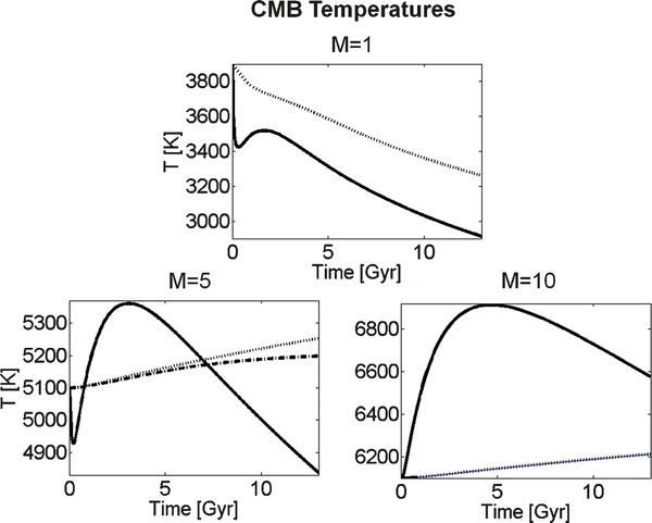
Figure 4. CMB temperatures as a function of time for M = 1, 5, and 10, and the viscosity models A (solid line), B (dotted), and C (dash-dotted) for the reference initial temperatures. For the M = 10 planet the CMB temperatures for models B and C are the same (dotted corresponds to the dash-dotted line for M = 10). Note that for our Earth-mass planet (M = 1) models B and C are based on the same effective activation volume V*eff = 2.5 cm3 mol−1, and hence do not differ.
Download figure:
Standard image High-resolution image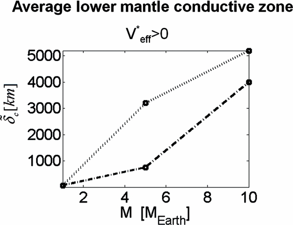
Figure 5. Thickness of the lower mantle conductive zone  averaged over 13 Gyr for the pressure-dependent models B (dotted) and C (dash-dotted) as a function of planetary mass for the reference initial temperatures. The variation with time is less than 15%. The pressure-independent model A leads to lower thermal boundary layers in the order of 1–10 km.
Download figure:
Standard image High-resolution image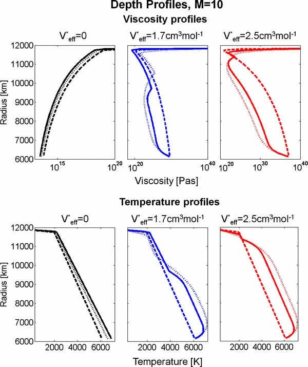
Figure 6. Viscosity and temperature profiles for an M = 10 super-Earth with Tc(0) = 6100 K for models A (black in the online journal), C (blue in the online journal), and B (red in the online journal) at different times: t = 0 Gyr (dashed), t = 4.5 Gyr (solid), t = 13 Gyr (dotted). The temperature profiles show the conductive heating in  due to internal heat sources, which lead to a deviation of the viscosity profile from a purely increasing or decreasing viscosity with depth. Note that we use different viscosity ranges for the V*eff = 0 and V*eff > 0 models for clarity.
Download figure:
Standard image High-resolution image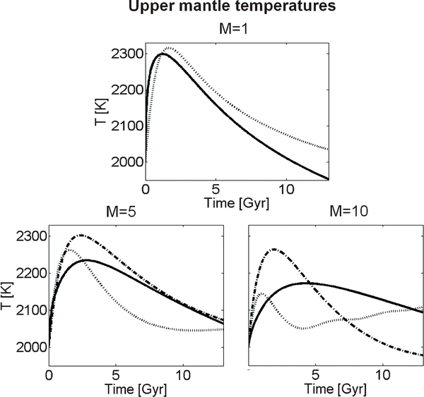
Figure 7. Upper mantle temperatures as a function of time for M = 1, 5, and 10, and the viscosity models A (solid line), B (dotted), and C (dash-dotted) for the reference initial temperatures. Note that for our Earth-mass planet (M = 1) models B and C are based on the same effective activation volume, and hence do not differ.
Download figure:
Standard image High-resolution imageFor the pressure-dependent models B and C a different thermal evolution can be observed depending on the planet's mass: for the Earth model (Figure 4, M = 1) pressure effects are relatively small, and we still observe a typical lower thermal boundary layer, which grows with the planet's cooling from 30 to 100 km in 13 Gyr. However, the effects of pressure on the viscosity are strong enough to reduce the convective vigor in the mantle. This is expressed by generally hotter interior temperatures in the mantle and core in comparison to model A (compare Figures 4 and 7 for M = 1). Nevertheless, independent of the effective activation volume V*eff, the M = 1 SL model predominantly cools with time (Figures 4 and 7).
With increasing planetary mass the cooling behavior differs significantly between the pressure-dependent and the pressure-independent models (Figures 4–7 for M = 5 and M = 10): we find a continuous, but slow heating of the core for both pressure-dependent models. The change in temperature is less than ∼50–150 K in 13 Gyr, leading to a negligible decrease in the CMB viscosity for models B and C with time (Figure 6). The heating of the core is the consequence of the conductive heating of the lower layer by the radiogenic heat sources. The core represents a large thermal reservoir without internal heat sources; hence the temperature in the lower mantle increases faster than in the core. Interestingly, for our pressure-dependent viscosity models the core does not heat up as fast as it does for V*eff = 0 in the first 2–5 Gyr. This can be explained by the observation that for the pressure-dependent models a large fraction of the lower mantle is conductively heated, distributing the energy produced by radiogenic heat sources over the whole lower mantle and the core. For V*eff = 0 the heat transport is more efficient due to vigorous convection and the energy is transported directly into two distinct thermal sinks, the upper mantle and the core, keeping the average lower mantle cooler than is the case for the pressure-dependent viscosity models (compare in Figure 6 the thermal profiles for V*eff = 0 with V*eff > 0).
The conductive zones in the lower mantle  occupy for the studied super-Earths and pressure-dependent models a large fraction of the planetary mantle. These conductive zones decrease with the initial phase of heating of the upper mantle in the first ∼3 Gyr (see Figure 7), and later grow with time as the upper mantle cools. The variation is, however, less than 15%, resulting in approximately constant
  thicknesses.
  increases in size with planetary mass and effective activation volume for pressure-dependent models (Figure 5 shows the thicknesses of
  averaged over 13 Gyr). The actual values are ∼4000 km and ∼5000 km for the M = 10 planet, and ∼700 km and ∼3000 km for M = 5 for models C and B, respectively.
The thermal evolution of the core for the pressure-dependent models B and C of the M = 10 planet is mainly independent of the convective mantle. A reduction of the effective activation volume, and hence an increase of convective vigor in the mantle from model B to C does not reduce the CMB and core heating, although the thickness of the lower mantle conductive zone is reduced by about 20%–40% (Figure 6). This effect is also attributed to the large thermal diffusion times in the thick conductive zones (see also discussion). Hence, the strong pressure-dependent viscosity thermally decouples the lowermost mantle and core from the convective mantle. This is different for the M = 5 planet, where pressure effects are weaker and a change from model B to C leads to a less efficient core heating by ∼30% (Figure 4).
Figure 6 shows the depth profiles of temperature and viscosity for an M = 10 planet with the three different viscosity models at three different times. Note that the adiabatic gradient depends on the upper mantle temperature Tm (e.g., see Stamenković et al. 2011), unlike in the classic linear approximation for smaller planets (e.g., Grott & Breuer 2008), and varies with time due to a change of Tm. Please further note that the innermost slope of the conductive thermal profile for models B and C (Figure 6) changes slowly with time due to the small thermal diffusion times. For larger thermal diffusivities (i.e., due to an increase of the thermal conductivity; see Section 6.4) this innermost slope diverges faster from the initial thermal slope.
For V*eff = 0, the initial phase of heating of the upper mantle is less efficient with increasing planetary mass, but at later times (>5 Gyr) more massive planets show higher upper mantle temperatures (Figure 7). This behavior can be explained by the initially stronger heating of the core for more massive planets as previously discussed (Figure 4)—less energy is available to heat the upper mantle at times before ∼3 Gyr. At later times (>3 Gyr) the super-heated core starts to cool and releases the stored energy. Due to the earlier stronger heating of the core with increasing mass more energy is available for larger planets to be released into the upper mantle.
The thermal evolution of the upper mantle is more complex when pressure effects are taken into account (Figure 7): for the pressure-dependent models B and C, the peak upper mantle temperatures still decrease with planetary mass. However, the general thermal evolution of the upper mantle is modulated by various factors. This complexity can be demonstrated for a specific planet with a fixed mass M and fixed initial temperature distribution considering an increase in the effective activation volume (i.e., comparing the viscosity model C with the viscosity model B for M = 10): the lower conductive zone in case of model B is thicker than in model C, and hence the effectively convecting mantle with the approximate thickness Deff ≈ Rl − Rb is smaller in comparison to model C. The thermal evolution of the upper mantle then crucially depends on (see Equation (12) and Figure 2):
- 1.the effective volume Ωeff of the convective mantle, which approximately scales as ∼Deff · A, with A being the average surface in the convective mantle,
- 2.the energy flux due to radiogenic heat sources in the fully convective region Deff, which scales as ∼Ωeff · Qm · A−1∼ Deff · Qm ∼ Deff,
- 3.the heat flux qm,in into this fully convecting zone out of
 , and
, and - 4.the heat flux out of the mantle qm,out,

which all strongly depend on the effective activation volume and the time-dependent ratio of the effective mantle thickness to the thickness of the conductive lower mantle zone  . The ratio reff decreases with increasing effective activation volume for a fixed planetary mass with the same initial thermal profile: in this case the heat flux into the convecting part of mantle qm,in generally increases due to a stronger heating of the conductive zone in the lower mantle
  , and the heat flux out of the mantle is reduced due to an increase in the thickness of the upper thermal boundary layer (indicating the reduced convective vigor in the upper mantle). This implies that for a specific planetary mass the upper mantle temperature Tm(t) should grow when the effective activation volume is increased. This is observed for intermediate pressure effects and smaller planets like our model Earth (Figure 7) when reff is still large.
For more massive planets additional effects complicate the thermal evolution of the upper mantle when the effective activation volume is further increased (comparing the viscosity model C with the viscosity model B for M = 5, 10 in Figure 7): reff strongly decreases, reducing the heat contribution due to radiogenic heat sources in Ωeff. This leads generally to cooler upper mantle temperatures for model B in comparison to model C. However, for M = 10 we observe after ∼7 Gyr (Figure 7) that the upper mantle temperature is again larger for the viscosity model B in comparison to the viscosity model C. This can be explained with the growth of the lower mantle conductive zone as well as the strong increase of the upper mantle SL thickness (L increases by a factor of three in 13 Gyr) with time, leading for the viscosity model B and M = 10 to a thin convective mantle (∼500 km). The effectively convecting mantle volume becomes so small that all incoming energy is directly converted into solely increasing Tm. This complex behavior also indicates that a simple scaling from planetary mass to the total heat flux is difficult when pressure effects of the viscosity are considered.
5.1.2. Variation of Initial Mantle and Core Temperatures
We first keep the reference initial CMB temperatures but increase the initial upper mantle temperature to the maximal peridotite solidus temperature in this zone, i.e., Tm(0) = 2300 K (see Section 4, Table 3): for all viscosity models the initially hotter upper mantle cools quickly and converges to the same upper mantle temperatures as for the initially cooler reference model—after about 2 Gyr the difference in upper mantle temperatures is less than 5% between the two models. This leads in the first ∼2 Gyr to a smaller conductive zone in the lower mantle by less than 25% for the initially hotter upper mantle model.
The impact of a varied initial upper mantle temperature on the thermal evolution of the core depends on the viscosity model and the planetary mass: the larger the lower mantle conductive zone (hence the more massive the planet or the larger the effective activation volume) the smaller is the impact from an initially hotter upper mantle on the lower mantle and the core. For both pressure-dependent models the initially hotter upper mantle heats the core additionally by ∼5%–30% during the entire evolution. For V*eff = 0 the thermal exchange between the upper mantle and the core is stronger, and we observe a stronger heating of the core during the first 2–5 Gyr. The maximal core heating is enlarged by about 40%–100%. However, due to the large CMB temperatures above 5000–6000 K this difference in core heating for all three viscosity models corresponds only to a small variation of the core temperature (<5%), which illustrates that the planet's dynamics is not strongly affected by the increase in initial upper mantle temperature.
The situation is different when varying the initial CMB temperature: with increasing initial CMB temperature the thickness of the lower mantle conductive zone  strongly decreases (Figure 8). For both super-Earth models (M = 5, 10) conductive zones in the lower mantle thicker than 500 km exist for initial CMB temperatures below ∼10,000–17,000 K for model B, and below ∼6000–12,000 K for model C, respectively. The decrease of the thickness of the lower mantle conductive zone with increasing initial CMB temperature reduces the efficiency of core heating and allows the core to start cooling above a certain initial CMB temperature (Figure 9). We find that the M = 10 planet starts to cool at initial CMB temperatures above ∼12,000 K for the viscosity model B and at initial CMB temperatures above 9000 K for model C. For the M = 5 planet and model B cooling starts at initial CMB temperatures of ∼7500 K; and for model C at initial CMB temperatures above ∼5600 K.
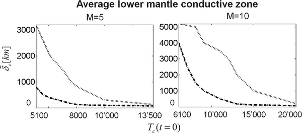
Figure 8. The lower mantle conductive zone  averaged over 13 Gyr as a function of initial CMB temperature Tc (t = 0). Model B with V*eff = 2.5 cm3 mol−1 is in dotted black, model C in dash-dotted black. For V*eff = 0,
  corresponds to a thin lower thermal boundary layer in the order of 1–10 km, which decreases with increasing CMB temperature due to the increase of convective vigor in the lowermost mantle.
Download figure:
Standard image High-resolution image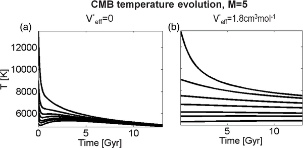
Figure 9. Evolution of the CMB temperature Tc(t) for the M = 5 planet in the stagnant lid mode for (a) viscosity model A and (b) viscosity model C for various initial CMB temperatures.
Download figure:
Standard image High-resolution imageFigure 9 shows the time evolution of the CMB temperature for the M = 5 planet and the viscosity models A and C with varying initial CMB temperatures up to the melting temperature of MgSiO3 perovskite at ∼570 GPa (∼13,500 K; Stamenković et al. 2011). For a pressure-dependent viscosity the cooling is much less efficient in comparison to V*eff = 0 even for high initial CMB temperatures. It is important to note that for the pressure-dependent models the CMB temperatures can differ by several thousand degrees kelvin after 13 Gyr (about 3000 K for the M = 5 planet in Figure 9) depending on the initial CMB temperature—the difference is much smaller without pressure dependence of the viscosity.
5.2. Plate Tectonics (PT) Regime
We examine the thermal evolution of planets with varying mass assuming the planets to be in the PT instead of the SL regime. PT increases the cooling rate of the upper mantle in contrast to SL convection, which results for pressure-independent rheologies also into an effective cooling of the core (Figures 10 and 11 for V*eff = 0; compare with, e.g., Breuer & Moore 2007). This is in contrast to SL convection where the deep interior remains comparatively warm as already suggested for smaller terrestrial planets (e.g., Breuer & Moore 2007).
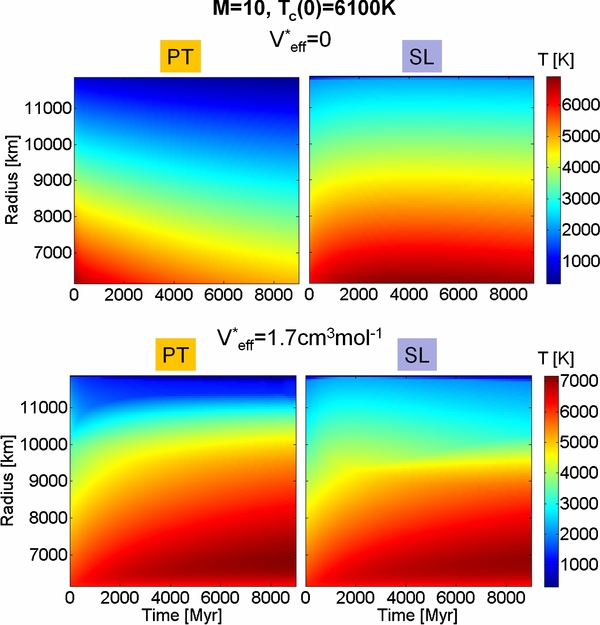
Figure 10. Radial mantle temperature distribution in (K) as a function of time in millions of years (Myr) for M = 10 and Tc(0) = 6100 K assuming the plate tectonics (PT) and stagnant lid (SL) mode with V*eff = 0 and V*eff = 1.7 cm3 mol−1.
Download figure:
Standard image High-resolution image
Figure 11. Interior temperature evolution for our Earth model (M = 1) with Tc(0) = 3900 K in a stagnant lid (SL) and a plate tectonics (PT) regime with V*eff = 0 and V*eff = 2.5 cm3 mol−1. For V*eff = 0 (V*eff = 2.5 cm3 mol−1) in solid black is the CMB temperature Tc; in dash-dotted black is Tb, the temperature at the upper border of  ; in solid gray is Tm, the upper mantle temperature; and in dash-dotted gray is Tl, corresponding to the temperature at the base of the stagnant lid for the SL regime or to the surface temperature Ts = 290 K for the PT regime. Compare with Figure 2.
Download figure:
Standard image High-resolution imageWith increasing V*eff and increasing planetary mass, however, we observe that the cooling behavior of the core and lowermost mantle becomes increasingly similar between the SL and the PT regime. This might be counterintuitive at first, but it reflects the ineffective convection of the lower mantle with increasing V*eff for both convection regimes. For super-Earths where CMB-lids are present, the core is even insulated by a conductive zone and hence not directly influenced by the convection in the upper mantle—and thus not affected by a change in the convective regime. This is shown in Figure 10 for the M = 10 planet with V*eff = 1.7 cm3 mol−1 and Tc(0) = 6100 K: in contrast to SL convection, PT leads to a stronger cooling of the upper mantle by about 600 K in 13 Gyr, and thus to an increase of the viscosity above the lower conductive zone  . As a consequence
  increases by about 10%, leading to an even better thermal insulation of the core. We observe this similarity in lower mantle and core cooling between the SL and the PT regimes for all studied super-Earths with viscosity models B and C, independent of initial CMB temperature (up to the melting temperature of MgSiO3 pv at the CMB). For smaller planets (below M = 1) or super-Earths with smaller effective activation volumes than suggested by model C the effects of pressure on the viscosity are smaller and we observe that PT can again more efficiently cool the core in comparison to SL convection.
Interestingly, with increasing effective activation volume the cooling of the core can become similar between an M = 1 planet in an SL and an M = 1 planet in a PT regime: for V*eff = 0 we observe a typical behavior where PT can much more effectively cool the core in comparison to SL convection (Figure 11). Independent of initial CMB conditions we obtain for V*eff = 0 and a PT Earth model a present-day CMB temperature of ∼2450 K, about 1300 K below the current estimate (see Kawai & Tsuchiya 2009; Stacey & Davis 2004; Tateno et al. 2009). The additional core cooling due to PT in comparison to SL convection is for V*eff = 0 about 760 K in 13 Gyr, for V*eff = 1.6 cm3 mol−1 it is 380 K, and for V*eff = 2.5 cm3 mol−1 the core cooling due to PT approaches the one caused by SL convection.
Note that for V*eff = 2.5 cm3 mol−1, i.e., the assumed effective activation volume at Earth's CMB for MgSiO3 perovskite (Stamenković et al. 2011), and a PT mode, the present-day CMB temperature is, for initial CMB temperatures up to 10,000 K, between 3550 and 3800 K. This value is similar to the current CMB temperature estimate of the Earth (see Kawai & Tsuchiya 2009; Stacey & Davis 2004; Tateno et al. 2009) in contrast to V*eff = 0 and active PT (∼2450 K). As a comparison: for V*eff = 0 our Earth model could only reach higher CMB temperatures if we model the Earth throughout 4.5 Gyr in the SL mode, but even then we obtain maximal CMB temperatures between 3300 and 3400 K today. This of course neglects the possibility of mantle layering as discussed later.
6. DISCUSSION
We have developed a 1D parameterized convection model to study the thermal evolution of super-Earths with a temperature- and pressure-dependent viscosity. Applying this model to super-Earths with varying planetary mass, and allowing them to be either in an SL or PT regime, we find that for pressure-dependent rheologies the initial thermal profile, in particular of the lower mantle, is crucial and controls the thermal evolution of the lower mantle and the core. The initial thermal profile is not well constrained and is most likely more complex and diverse than assumed in our study. However, even if the planet starts as completely molten, it is likely that due to low viscosities the interior first strongly cools down but quickly approaches a regime where pressure effects start to reduce the cooling and convective vigor for V*eff > 0. This is supported by our results that even with initial CMB temperatures close to the melting temperature of MgSiO3 pv the associated cooling results rapidly in a sluggish convection of the lower mantle and in a reduced core cooling.
The dependence of the thermal evolution on the initial thermal conditions is only minor for V*eff = 0. Even for SL planets the interior temperatures converge after a few Gyr, independent of the initial state (see Figures 9 and 12). This self-regulation of the average mantle temperature is the so-called thermostat effect and is often used to infer the thermal structure of planets. The thermostat effect is due to the strong temperature dependence of mantle viscosity and due to vigorous convection when pressure effects are minor (Tozer 1967): for a hot planet, mantle viscosity is low and extremely vigorous convection rapidly cools the planet. For a relatively cool planet, the mantle viscosity is higher and convection cools the planet at a reduced rate. Self-regulation tends to bring the viscosity of the mantle to a value that facilitates efficient removal by convection of the heat generated in the mantle. It is even possible that an initially cold mantle would heat up by radioactivity until the self-regulated viscosity is reached. As a consequence of the self-regulation, the present state of the convecting mantle has little or no memory of the initial conditions for V*eff = 0 (Figure 12). However, for V*eff = 0 the thermostat effect is more efficient for PT planets than for SL planets (Figure 12), which is due to the fact that the SL additionally insulates the mantle and prohibits effective cooling.

Figure 12. CMB temperature Tc as a function of time for the non-pressure-dependent viscosity model with V*eff = 0 for different initial CMB temperatures, up to the CMB melting temperature of MgSiO3 perovskite (Stamenković et al. 2011) for PT and SL planets. For M = 1: Tc(0) = 3900 K and 5700 K. For M = 10: Tc(0) = 8100 K, 13,000 K, and 20,000 K.
Download figure:
Standard image High-resolution imageFor massive and ''cooler'' planets (with interior temperatures as discussed in the literature, i.e., Papuc & Davies 2008, Sotin et al. 2007, and Valencia et al. 2006) we find that large conductive zones can exist, suggesting a large partially stagnant mantle (compare with Section 6.1). These conductive zones insulate the core and lead predominantly to a steady core heating in case of both SL and PT convection on super-Earths.
It is important to note that for the cases where a large lower mantle conductive zone is present conductive heating due to radiogenic heat sources is not efficient enough to sufficiently reduce the lower mantle viscosities with time for convection to operate in the deep mantle (compare with Section 6.1 where we explicitly demonstrate the existence of CMB-lids and their similarity to the 1D lower mantle conductive zones  ). This is at first intriguing as the ''steady-state'' interior temperatures for a lid with a thickness in the order of ∼1000 km and our standard radiogenic heat source concentration are found to be above ∼20,000 K. The slow heating of the lower mantle can be partially explained by a large diffusion time, which is a measure for the time necessary to reach this steady-state when the boundary temperatures are held constant. Please note that we study a dynamical case where the boundary temperatures are changing with time; hence diffusion times are only approximate indications for the effectiveness of conductive heating. For a conductive lid with the thickness Dcond, the diffusion time scales like:

For a lid of ∼1000 km thickness and our reference thermal conductivity of about ∼4 W m−1 K−1 this leads to diffusion times of ∼60–70 Gyr for super-Earths between 5 and 10 Earth masses. The thermal conductivity has to increase by at least a factor of ∼60 to reduce the diffusion time below 1 Gyr and to make it geologically relevant. For our standard thermal conductivity the diffusion time is less than ∼500 Myr if the conductive structures are smaller than ∼100 km, and the steady-state can be reached in geological times.
6.1. 2D Convection Results and Comparison with the 1D Model
The 1D model is a first approach to modify classic parameterized 1D convection models by including strong pressure effects on the viscosity. In the following, we compare the 1D results with those of a 2D spherical convection model to examine whether our approach can describe satisfactorily the thermal evolution with temperature- and pressure-dependent viscosity. It is not aimed to derive or adjust the parameterization from the 2D results as this requires a substantial study far beyond the scope of this paper.
We have performed a variety of 2D spherical convection simulations assuming the Boussinesq approximation and compare them with our 1D parameterized calculations. We use the same parameters as in the reference model for the 1D runs (Tables 1–4) apart from the reference viscosity and the initial temperature profile to sustain numerical stability. Details of the 2D convection model including the chosen parameters are described in Appendix B and in Table 5.
Table 5. 2D Results for the Standard Thermal Profile (see Appendix B)
| 2D Runs | ||||||
|---|---|---|---|---|---|---|
| M | V*eff | ηref | TC(0) | TC(4.5/13) | LC(4.5/13) | LT(4.5/13) |
| (MEarth) | (cm3 mol−1) | (Pa s) | (K) | (K) | (km) | (km) |
| 10 | 2.5 | 1021 | 6100 | 6130/6152 | 5635/5635 | 0/0 |
| 10 | 1.7 | 1022 | 6100 | 6130/6152 | 4680/3862 | 955/1773 |
| 10 | 1.7 | 1021 | 6100 | 6130/6152 | 3681/3226 | 1000/2409 |
| 5 | 2.5 | 1023 | 5100 | 5146/5189 | 4600/2781 | 0/1819 |
| 5 | 2.5 | 1023 | 6100 | 6118/6125 | 3523/2781 | 1077/1819 |
| 5 | 2.5 | 1022 | 5100 | 5148/5189 | 2633/1743 | 964/2857 |
| 5 | 1.8 | 1024 | 5100 | 5146/5189 | 3152/0 | 1448/3597 |
| 1 | 2.5 | 1025 | 3900 | 3984/3871 | 0/0 | 69/1875 |
Notes. At different times t = 0 Gyr, 4.5 Gyr, and 13 Gyr (corresponding to the numbers in parentheses) for a planet with relative Earth mass M, effective activation volume V*eff, and reference viscosity ηref. Tc is the CMB temperature, Lc is the thickness of the CMB lid, and LT is the thickness of the transitional lid—note that both lids are computed based on laterally averaged Pe profiles. For mantle thicknesses compare with Figure 1.
Download table as: ASCIITypeset image
To distinguish the convective and stagnant regions in the 2D model, we use the Peclet number, Pe, which is the ratio between the energy transported by convection and by diffusion, Pe = uD/κm with u being the velocity, D the mantle thickness, and κm the thermal diffusivity. For Peclet numbers smaller than one, convection velocities are almost zero and we define the region to be stagnant.
We further distinguish between transitional and convective regions. For Peclet numbers between 1 and 100 the convection is highly sluggish (depending on planetary mass Pe = 100 corresponds to mantle velocities below 0.1–1 mm yr−1). The effectively convecting region is defined for Pe numbers larger than 100. The laterally averaged values for the CMB-lid and transitional lid thicknesses have to be considered with care as information about local partial stagnant zones might be lost, or as very low convective velocities might be associated with a zone where, based on our definition, no stagnant (CMB) lid exists.
All 2D convection models confirm the formation of a stagnant lower mantle zone, a CMB-lid, during the thermal evolution of super-Earths with 5 or 10 Earth masses for the reference temperatures. The CMB-lid thickness is found to increase strongly with planetary mass, effective activation volume, and reference viscosity, and to decrease for larger interior temperatures as suggested already by the 1D models. For our Earth model (M = 1) stagnant zones at the CMB are not present but small transitional zones are observed assuming a relatively high reference viscosity of 1025 Pa s (Table 5; note that the transitional zones would decrease if we assume a more appropriate reference viscosity of 1021 Pa s).
In the following, we show the most significant 2D results for M = 5 and M = 10 planets at times when the convective vigor peaks as well as after 13 Gyr of thermal evolution to illustrate the general convective behavior assuming pressure-dependent viscosity in the mantles of super-Earths (Figures 13 and 14). Note that for convection to start it takes up to 1–3 Gyr depending on initial thermal profile and reference viscosity.

Figure 13. 2D simulation results for M = 10, Tc(0) = 6100, ηref = 1021 Pa s, and V*eff = 1.7 cm3 mol−1 with the standard initial thermal profile (Appendix B). Panels (a) and (d) show the 2D temperature (K), (b) and (e) the convective velocities (cm yr−1; black represents convective velocities below ∼0.01 cm yr−1), and (c) and (f) the regions with the Peclet number below 1, in between 1 and 100, and above 100—indicating stagnant, sluggish, and effectively convecting zones, respectively. Panels (a)–(c) show results at t = 7.5 Gyr and (d)–(f) at t = 13 Gyr. The convective velocity peaks at ∼7.5 Gyr with ∼3.5 cm yr−1. In the velocity pictures the average convective velocity in the black zone is negligible with ∼10−6 cm yr−1. The central gray-filled circle is the planet's core.
Download figure:
Standard image High-resolution image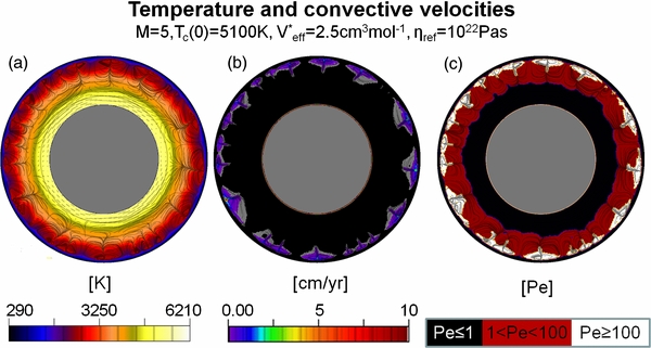
Figure 14. 2D simulation results for M = 5, Tc(0) = 5100, ηref = 1022 Pa s, and V*eff = 2.5 cm3 mol−1, and the standard initial thermal profile (Appendix B) at the peak of convection around t = 7.5 Gyr. (a) The 2D temperature (K), (b) the convective velocities (cm yr−1), and (c) the regions with the Peclet number smaller than 1 (black), between 1 and 100 (red), and above 100 (white)—indicating stagnant, sluggish, and effectively convecting zones, respectively. The central gray-filled circle is the planet's core.
Download figure:
Standard image High-resolution imageFigure 13 shows an M = 10 planet with standard initial temperatures and a reference viscosity of 1021 Pa s. The convective velocities reach a maximum of ∼3.5 cm yr−1 at ∼7.5 Gyr and decrease to maximal ∼0.5 cm yr−1 after 13 Gyr of evolution. The CMB-lid comprises more than ∼60% of the entire mantle and the CMB heats slowly by ∼50K during 13 Gyr, indicating the conductive heating of the lower mantle and core as observed and discussed for the 1D model. Although the uppermost mantle convects, we find for all studied M = 10 cases, independent of the chosen initial upper mantle or CMB temperature (see Appendix B), that a transitional zone comprises almost the whole convecting mantle, indicating a generally sluggish convection for the M = 10 planet. This is indicated by the rather low convective velocities thoughout the planet's mantle (Figures 13(b) and (e)).
The M = 5 planet shows more vigorous convection in comparison to the M = 10 planet. Figure 14 shows results for a 5 Earth mass planet and V*eff = 2.5 cm3 mol−1, Tc(0) = 5100 K, and ηref = 1022 Pa s at t = 7.5 Gyr, when the convection is strongest. For this case we find thinner CMB-lids, which comprise about 40% of the entire mantle, and a transitional zone that comprises about 70% of the non-stagnant mantle.
Our 2D results show that for the suggested temperature- and pressure-dependent rheologies and the standard temperature profiles convection strength in super-Earths decreases with planetary mass, leading to a stagnant lower mantle and to a highly sluggish convection above large CMB-lids (Table 5).
As described in Appendix B, we have performed additional runs with CMB temperatures increased by 1000–2000 K, as well as runs with an initially hotter upper and/or hotter average mantle. But even here we generally find a strong reduction of convective vigor for more massive planets as well as increasing CMB-lids with planetary mass. For those initially hotter planet models we specifically find the following results, which are all in excellent agreement with our 1D model:
- 1.An increase of CMB temperature (2000 K for M = 10, 1000 K for M = 5) does not significantly affect the thickness of the CMB-lid or the transitional lid.
- 2.An initially hotter upper mantle (by reducing the initial upper thermal boundary layer thickness, see Appendix B) does not significantly affect the CMB-lids, although it helps to earlier ignite upper mantle convection.
- 3.An initially hotter average mantle (by increasing the initial intermediate mantle temperature with planetary mass, see Appendix B) contributes in reducing the CMB-lid thicknesses, but still results in large transitional lids, which comprise a significant fraction of the convective mantle.
The results of the 2D and 1D models are in good agreement. In particular, the thermal profiles in the lower mantle and the CMB temperatures are very similar between the two models for M = 5 and M = 10: for instance, the difference in core heating assuming the reference temperatures is less than 10% and the CMB temperatures differ by no more than 2% at all times during 13 Gyr.
The thermal profiles, however, differ in the upper part of the lower mantle conductive zone and the uppermost convective mantle (Figures 15(a) and (c)). This difference can be explained by the assumption made for the 1D model that the zone above  is adiabatic (isothermal) between the thermal boundary layers and by not separating the lower thermal boundary layer and the CMB-lid. The first assumption, i.e., the convective temperature profile in our 1D model being adiabatic, implies a vigorously convecting mantle layer. Note that we use the Boussinesq approximation in the 2D model, which neglects adiabatic effects and viscous heating, and results in an almost isothermal convecting zone when the convection is vigorous. A comparison between the 2D and the 1D model, which intrinsically accounts for an adiabatic gradient, indicates that the Boussinesq approximation in the 2D model underestimates lower mantle temperatures. This temperature underestimation is not significant, indicating that the Boussinesq approximation can be used as a first step (e.g., O'Neill & Lenardic 2007; Stein et al. 2011). A more detailed analysis is required to account for the adiabatic and viscous effects in the 2D model, but is beyond the scope of this work. For a direct comparison with the Boussinesq approximated 2D model, we adjust our corresponding 1D model calculations by assuming that the adiabatic temperature increase in the convecting zone is negligible, and thus is isothermal. The 2D thermal profile shows an isothermal upper mantle at the time of strongest convection (Figure 15(a)) but later in time the temperature increases with depth across the upper mantle due to sluggish convection (Figure 15(c)). Thus, the 1D model overestimates the convective vigor in the convecting zone (above
  ) as we always assume strong, non-sluggish convection in this layer.

Figure 15. Viscosity and temperature profiles for 1D (gray) and 2D models (black; solid for average, dashed for minimal, and dotted for maximal values of temperature or viscosity in each shell). For the same planet model shown in Figure 14 with M = 5, Tc(0) = 5100, ηref = 1022 Pa s, V*eff = 2.5 cm3 mol−1, and the standard initial thermal profile at different times: (a) and (b) t = 7.5 Gyr, when convection is strongest, and at (c) and (d) t = 13 Gyr.
Download figure:
Standard image High-resolution imageThe conductive behavior in the lower mantle is on the other hand overestimated in the 1D model because we cannot separate the lower thermal boundary layer and the CMB-lid. This leads to a smaller cooling of the lower mantle in the 1D model compared to the 2D model but the difference is comparatively small. In addition, a direct comparison between the CMB-lid based on the 2D model and the 1D lower thermal conductive zone  is difficult. Nevertheless, we find that
  is always in between the 2D CMB-lid and transitional lid, increases with planetary mass, effective activation volume, and reference viscosities, and decreases with interior temperatures in a similar manner as observed with the 2D model.
Although the differences in the results between the 1D and 2D models can be relevant for a detailed study of the thermal evolution of super-Earths, we find that the general thermal trends, in particular of the lower mantle and the core, are represented satisfactorily with the 1D model. Being aware of the 1D model's limitations (see also below), we can use it to discuss general consequences of a pressure-dependent viscosity on the thermal evolution of super-Earths.
6.2. Limitations of the 1D Model and the Interpretation of

In the following, we want to address some limitations of the 1D model and their possible impact on our findings. The critical Rayleigh number based on the viscosity contrast (Equation (25)) was derived for monotonically increasing or decreasing viscosities (Figure 3). For some cases, however, we find that due to radiogenic heating in the conductive zone of the lower mantle  the viscosity profile deviates with time from a monotonic behavior (Figure 6). This deviation shifts the actual minimum of the viscosity profile to greater depths below Rb and leads to an effectively larger viscosity contrast of this subsystem. We performed all runs adjusting for this viscosity shift with time to greater depths, by using for the calculation of
  (Equation (26)) the minimal viscosity of the layer as the characteristic viscosity of the system instead of the viscosity at Rb as well as the maximal viscosity contrast of the layer to calculate Racrit(Δη). We find that the increase of the viscosity contrast due to this shift compensates the effects of the reduced characteristic viscosity of the system. Thus, the thermal evolution does not significantly differ (deviation in Tm and Tc is less than 1%), although
  is reduced by ∼10%–50% and shows a generally stronger decrease with time. We hence conclude that this deviation is not large enough to change the thermal trends observed by our model. In addition, we have to be aware that classic Rayleigh numbers are defined for a linear temperature increase, which is due to conductive heating of the lower mantle not any longer given (see Figure 6). However, we find this deviation to be small, and observe no essential change of the thermal evolution if we use the maximal temperature contrast of the system instead of ΔT = Tc − Tb. Note that the deviation from a linear temperature increase is smaller considering also the depth dependence of the thermal conductivity. In this case, the lower mantle cools more effectively and the thermal profile in the lower mantle conductive zone becomes increasingly linear, leading to a monotonically increasing or decreasing viscosity (see Section 6.4).
The results of the 2D model with a thick CMB-lid (e.g., Figures 13–15) indicate that convection in the upper mantle is sluggish in contrast to what we assume in the 1D model. An overestimation of the convective strength is also possible when the conductive layer at the CMB is thin due to high CMB temperatures. This scenario is illustrated in Figure 16 and occurs for the pressure-dependent models B and C at initial CMB temperatures above ∼8000 K and 9000–11,000 K for the M = 5 and the M = 10 planets, respectively. For these cases, the viscosity contrasts in the convective adiabatic layer above  are between 105 and 1010 and the absolute viscosities can reach values between 1025 Pa s and 1035 Pa s—conditions not favorable for convection in the zone above
  (the red zone in Figure 16 in the online journal).
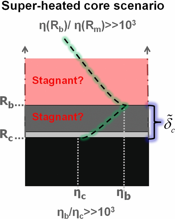
Figure 16. Viscosity profile (dashed) for a temperature- and pressure-dependent viscosity (models B and C) of a scenario with a super-heated lowermost mantle and core in comparison to the remaining mantle, which occurs when the initial CMB temperatures are high (Tc(0) > 8000–11,000 K depending on planet mass and effective activation volume; compare with Figure 9) and when the pressure effects on the viscosity are large (model B for M = 5, models B and C for M = 10). For these cases, the viscosity strongly decreases with depth through  , leading to a large viscosity contrast through this rather small lower mantle conductive zone on the order of a few ∼100 km (Figure 8). The viscosity and viscosity contrasts through the adiabatic mantle above
  (red in the online journal) are large, indicating stagnant zones. The zone with the lowest viscosity in
  , which should indicate the lower thermal boundary layer, is shown in light gray and is at the bottom of
  .
.
Download figure:
Standard image High-resolution imageThis, on the other hand, suggests that the cooling of the interior might be less efficient than predicted by our model. In addition, in this super-heated core scenario (Figure 16) the stability of the conductive layer  at the CMB is difficult to predict: the viscosity decreases with pressure across the conductive layer and the viscosity contrasts can reach ∼10 orders of magnitude, but the least stable part of
  is at its bottom where the viscosity is minimal. This suggests that the uppermost part of
  is stagnant and that the lowermost part of
  may be unstable.
In the present 1D model, we do not distinguish between the lower thermal boundary layer and the CMB-lid. This introduces an error into the energy conservation equation of the mantle (Equation (12)) as we underestimate the volume and hence the amount of radiogenic heat sources in the convective zone. As shown by Stengel et al. (1982) the viscosity-contrast-dependent critical Rayleigh number used to determine  (Equation (25)) can be partially explained by assuming that the lower thermal boundary layer's thickness is described by
The constant c depends on the viscosity law (compare with Solomatov 1995). For a viscosity exponentially decreasing with temperature Stengel et al. (1982) find that c = 8, and hence Equation (28) suggests that the lower thermal boundary layer comprises only a fraction of the lower mantle conductive zone if the viscosity contrast through  is above ∼3 × 10³. Adjusting the energy equations (Equation (12)) to include δc as part of the convective mantle using Equation (28), we find qualitatively the same trends as observed without a direct determination of the lower thermal boundary layer. We have modeled several cases accounting for this correction and find that in comparison to the standard 1D model the upper mantle is maximally ∼150 K (∼5%) hotter due to the larger amount of heat sources in the convective zone. This leads to stronger core heating or smaller core cooling rates, respectively. For the reference model the core is up to ∼50 K hotter after 13 Gyr of evolution for the pressure-dependent models B and C. As an additional consequence of the hotter convective mantle, the total lower mantle conductive zones are about 5%–15% smaller.
However, we find that the CMB-lids predicted by Equation (28) for the 1D model are a factor of two smaller than those suggested by 2D models for the same cases. Moreover, although it has been shown that the viscosity contrast through the upper thermal boundary layer is smaller than one order of magnitude (e.g., Davaille & Jaupart 1993) we do not obtain the same viscosity contrast through δc estimated with Equation (28). Instead we find that the viscosity contrast through the suggested lower thermal boundary layer starts initially at ∼103–104. For our reference model and massive planets with large CMB-lids such as the M = 10 super-Earth with V*eff = 2.5 cm3 mol−1 this viscosity contrast falls after 5 Gyr below one order of magnitude. For less massive planets or weaker pressure effects the viscosity contrast is only after ∼10 Gyr below one order of magnitude. This might suggest that the viscosity contrast through the lower thermal boundary layer reaches one order of magnitude in the steady-state. Our results, however, indicate that this limit cannot be reached in geologically relevant times.
Interestingly, the comparison between 2D and 1D CMB-lid thicknesses is far better when the constant of c ∼ 8 in Equation (28) is reduced to c ∼ 1. In this case the viscosity contrast through δc is closer to one order of magnitude, indicating that the lower thermal boundary layer, which is effectively taking part in the convection, is for our viscosity law indeed smaller than suggested by Equation (28). Future studies are required to better constrain the thickness of the lower thermal boundary layer associated with a temperature- and pressure-dependent Arrhenius-type viscosity.
6.3. Sensitivity to the Characteristic Rayleigh Number
The 1D model assumes that the characteristic Rayleigh number defining the lower mantle conductive zone equals the viscosity-contrast-dependent critical Rayleigh number  . To test the sensitivity of our results on the critical Rayleigh number, we additionally perform all runs with a constant value for
  , setting it to our isoviscous value of
  —corresponding to a lower limit of the possible values of
  .
.
The main differences between a constant characteristic Rayleigh number model and our standard viscosity-contrast-dependent model are illustrated in Figure 17: for the standard reference temperatures we find almost no differences in the thermal evolution (the CMB temperature Tc(t) and the upper mantle temperature Tm(t) vary by less than 1% between the two models). The differences increase for larger initial CMB temperatures and smaller planets. Here we find smaller lower mantle conductive zones (by 5%–30%) and an increase of cooling rates (see Figure 17(a) for M = 5 in an SL mode, and Figure 17(b) for M = 1 in a PT mode). For super-Earths the core starts cooling at 100–1000 K lower initial CMB temperatures than for  , but nonetheless cooling is far less effective than for V*eff = 0.

Figure 17. (a) CMB temperature evolution Tc(t) for the M = 5 planet in the stagnant lid mode for model C (V*eff = 1.8 cm3 mol−1) for various initial CMB temperatures with  . Compare with Figure 9 where
  . (b) The interior temperatures for our M = 1 model (see Figure 2) in a PT regime with V*eff = 2.5 cm3 mol−1 for the two different Racrit models and reference initial temperatures. For our standard Racrit model (see Figure 11): in solid black, we give the CMB temperature Tc and in dash-dotted black we give the temperature Tb at the upper border of
  ; in solid dark gray, we show the upper mantle temperature Tm and in dash-dotted dark gray we show the surface temperature. In light gray are the results for
  ; there are no differences in the upper mantle between the two Racrit models. For
  the CMB temperature today would be ∼3150 K, about 450 K cooler than for a corresponding SL model, but still ∼700 K hotter than for a PT model withV*eff = 0.
Download figure:
Standard image High-resolution imageIn conclusion, the difference between 1D thermal evolution models with  and
and  is not significant and all observed thermal trends and effects remain unaltered. These results indicate that the viscosity controls substantially the dynamics and the thermal evolution.
6.4. The Pressure and Temperature Dependence of αm, km, and ρm
In the models presented we investigate the effects of a temperature- and pressure-dependent viscosity on the thermal evolution of super-Earths, but we neglect any temperature and pressure dependence of the thermal mantle conductivity km, the thermal mantle expansivity αm and the mantle density ρm.. Their change with depth, due to pressure and temperature, is however smaller compared to the variation of the mantle viscosity with depth.
To test the impact of an additional variation of km, αm, and ρm with temperature and pressure, we proceed to compute the upper thermal boundary layer, the upper mantle SL, and the heat flux out of the mantle as before with standard values for km, αm (Table 1), and the average mantle density ρm. However, for the lower mantle, i.e., for the computation of the lower mantle conductive zone (Equation (26)), the lower mantle conductive zone heat equation (Equation (23)), and the heat flux into the mantle and out of the core (Equations (21) and (22)) we distinguish two simplified test cases:
- 1.We use higher km values for the lower mantle (varied from the standard value of km = 4 W m−1 K−1 to 20 W m−1 K−1 and 40 W m−1 K−1) but keep our standard αm and the average mantle density ρm.
- 2.We use the results from Stamenković et al. (2011), who computed km, αm, and ρm for an Earth-like 80 vol.% MgSiO3 perovskite and 20 vol.% MgO periclase mantle composite (in fact we assume periclase to only significantly alter the phonon thermal conductivity), and use for every time step of the thermal evolution average values of km, αm, and ρm evaluated at the average temperature and pressure in.

We generally observe that with increasing thermal conductivities the lower mantle cools more efficiently, leading to larger  due to the larger viscosity. This results in an increasingly linear temperature profile in this zone (Figure 18 for M = 10 in an SL mode). However, the more efficient cooling of the lower mantle does not imply a stronger cooling of the core. In fact, with increasing thermal conductivity heat is transported also more efficiently into the core, which results in an even stronger heating of the core (Figure 18). There is, however, a threshold, i.e., increasing the thermal conductivity of the lower mantle above a critical value would cause the core to only cool. For the chosen example in Figure 18 this critical conductivity is ∼100 W m−1 K−1, which is about four times larger than the thermal conductivity suggested by Stamenković et al. (2011) for the corresponding pressure and temperature regime.
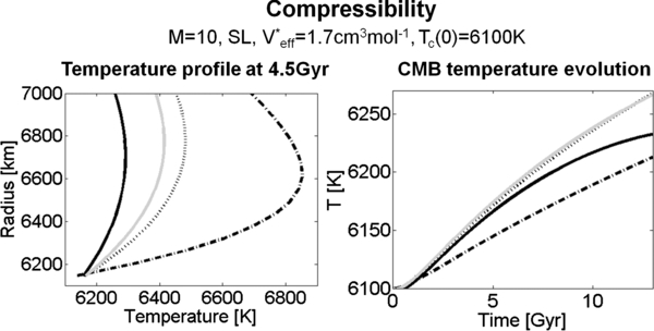
Figure 18. For a 10 Earth mass super-Earth in a stagnant lid regime with V*eff = 1.7 cm3 mol−1 and Tc(0) = 6100 K: temperature profile in the lowermost mantle at t = 4.5 Gyr and the CMB temperature as a function of time for models with varied total thermal conductivity km, thermal expansivity αm, and density ρm. The model with km = 4 W m−1 K−1 is in dash-dotted black (standard); with km = 20 W m−1 K−1 in dotted black; with km = 40 W m−1 K−1 in solid black; and with km, αm, and ρm from Stamenković et al. (2011) in solid gray.
Download figure:
Standard image High-resolution image
The results of Stamenković et al. (2011) suggest for the specific M = 10 planet (Figure 18) that the average total thermal conductivity in  (phonon + radiation + electrons) is about 20–25 W m−1 K−1 (5–6 times larger than our standard value of 4 W m−1 K−1), that the average thermal expansivity is ∼4 × 10⁻⁶ K−1 (∼5 times smaller than our standard value) and that the average density in
  is similar to the average mantle density ρm. We find the effects of the five-times-smaller thermal expansivity to be minor compared to the effects of the five-times-larger thermal conductivity in comparison to our standard model. The model with varied km, αm, and ρm is similar to the km = 20 W m−1 K−1 model in Figure 18. This is due to the fact that the thermal expansivity only affects the thickness of the lower mantle conductive zone
  (Equations (24) and (26)), but the thermal conductivity governs as well the heat transport through
  (Equation (23)), the heat flux out of the core (Equation (22)), and the heat flux into the convecting mantle (Equation (21)).
In general, we conclude that the temperature and pressure dependence of km, αm, and ρm only strengthens our conclusion that a stagnant layer at the CMB can be present in super-Earths. In particular, higher values of the thermal conductivity in the lower mantle result in more efficient cooling of the lower mantle and hence lead to increasing  . This even further supports the idea that heat in the deep interior of super-Earths is transported via conduction rather than by convection for lower initial interior temperatures.
6.5. Implications for the Propensity of Plate Tectonics and the Magnetic Field Generation
The propensity of super-Earths to have PT has been controversially discussed in the recent past (Korenaga 2010; O'Neill & Lenardic 2007; Stein et al. 2011; Valencia et al. 2007; Valencia & O'Connell 2009; Van Heck & Tackley 2011). In these models, the pressure dependence of the viscosity is generally neglected and it is assumed that the entire mantle convects vigorously. Our present models show that if the pressure dependence of the viscosity is considered the effectively convecting mantle can be significantly reduced in thickness depending on initial conditions. Hence, one can also expect the propensity of PT to be affected, which is influenced, among other factors, by the yield stress τy and the convective shear stress τc beneath the lithospheric plate of thickness L. A necessity for PT is plate yielding, which can only be achieved when the convective stress overcomes the yield stress of the lithospheric plate. Due to the fact that for V*eff > 0 we generally observe a reduction of convective vigor with increasing planetary mass, as well as a reduction of convective mantle thickness, the mantles of super-Earths with large enough CMB-lids resemble in their convective structure actually less massive planets. Assuming that for V*eff = 0 less massive planets have smaller chances of driving PT, as has been suggested by Valencia et al. (2007), would lead to the conclusion that for massive super-Earths the propensity of PT could start to decrease with increasing mass. Interestingly, O'Neill & Lenardic (2007) suggest a decrease of surface mobility for super-Earths already for viscosities with nearly V*eff = 0 and Stein et al. (2011) even for a decrease in lower mantle viscosity due to a change of diffusion mechanism from vacancy to interstitial control as suggested by Karato (2011). However, as already discussed, for V*eff > 0 the convective structures in super-Earths strongly depend on the planet's initial conditions and hence it might be difficult to obtain a relation between the propensity of PT and the planetary mass.
Moreover, independent of viscosity law and the mass of the planet, the propensity of PT might be even stronger influenced by the amount of volatiles, i.e., water in the lithosphere, the age of the planet, lithospheric buoyancy as suggested by Kite et al. (2009), and most of all by the amount of radiogenic heat sources, which might crucially vary from planet to planet and could as well depend on the time of planetary formation in relation to the age of the universe.
Classic dynamo generation requires convection in a partially liquid metallic core by thermal or compositional buoyancy, which on the other hand requires that the core is cooling (for a description of thermal and compositionally driven dynamos, see, e.g., Stevenson 2009). The present results indicate that core cooling in super-Earths is strongly reduced for pressure-dependent rheologies. In fact for our reference models, assuming temperatures that are currently suggested for super-Earths (Papuc & Davies 2008; Sotin et al. 2007; Valencia et al. 2006), the core is continuously heating—preventing dynamo generation for these cases. For higher initial temperatures, the core may cool with time but possibly with a heat flux below the critical heat flux necessary for driving a thermal dynamo. Such behavior is already discussed by Tachinami et al. (2011) for super-Earth conditions with an olivine rheology. However, this does not generally exclude chemical dynamo generation, for which the growth of a solid iron core could induce convection and hence a magnetic field—in that case the core also needs to cool, but the rate can be smaller than for a thermal dynamo and the core temperature needs to be partially (but not completely, see below) under the liquidus of the iron-rich core. Moreover, the steep melting curves for MgSiO3 perovskite and MgO by Stamenković et al. (2011) associated with large effective activation volumes for mantle rock also indicate large melting gradients for iron. Hence, additionally, the melting temperatures of iron could strongly increase with pressure and make it more difficult for more massive planets to have molten iron cores, a necessity for dynamos. Thus, although we cannot exclude magnetic field generation in super-Earths, assuming a temperature- and pressure-dependent viscosity strongly limits the conditions preferable for dynamo action to a small parameter range. Note that this conclusion does not change if the planet is in the PT regime (compare with Section 5.2).
6.6. Observables and Volcanism on Super-Earths
Present observations of super-Earths are mainly limited to mass and radius and do not provide direct information on interior dynamics. The atmospheric chemistry, however, which could be investigated by combined future observations (as with Spitzer, Hubble, the possibly upcoming EChO mission, or with the James Webb Space Telescope), is influenced by the planet's outgassing history and volcanism—with both being affected by the interior composition, structure, and rheology.
If the viscosity is strongly pressure-dependent then super-Earths might be even undifferentiated, i.e., no separation of an iron core and a silicate mantle, as indicated by Stamenković et al. (2011)—note that for this study we assume that differentiation took place. An undifferentiated interior would lead to a potentially different outgassing history, and hence atmospheric composition, in comparison to a differentiated body, which is more likely to form when the effective activation volume is small.
Assuming, however, a differentiated interior, we find that for SL planets melt production decreases with both increasing planetary mass and effective activation volume, indicating a reduced volcanic activity for SL super-Earths in comparison to an SL M = 1 planet. Using the peridotite solidus data from Hirschmann (2000), the duration of upper mantle melt production for SL planets decreases with planetary mass for V*eff = 0: melt production is possible for an M = 1 planet until 9 Gyr after the planet's formation, but an M = 10 super-Earth can produce melt only during the first 6 Gyr. This reduced duration of melt production for V*eff = 0 with increasing planetary mass can be mainly explained by the increase of gravity that enlarges the radial gradient of the melting curve, and additionally by the decreasing peak upper mantle temperatures for larger M (see Figure 7).
An increase of the effective activation volume does not severely alter the upper mantle temperature for a specific planet (see Figure 7) but leads to a strong increase of the SL thickness for super-Earths (when V*eff is increased from V*eff = 0 to V*eff = 2.5 cm3 mol−1 the lid thickness L for M = 1 is almost unaltered, but for M = 5, 10 L increases by a factor of two or four, respectively. This is due to the higher viscosity, which is a consequence of the increased pressure effect). This leads to an additional reduction of the thermal gradient in the upper mantle for M = 5, 10 planets in comparison to V*eff = 0, hence melt production in the upper mantle is even more suppressed for increasing V*eff. For M = 5 and M = 10 melt in the upper mantle can only be produced during the first 4 Gyr or the first 1 Gyr, respectively. A basal magma ocean seems unlikely due to the large MgSiO3 perovskite and MgO melting temperatures found by Stamenković et al. (2011).
Hence if super-Earths are more likely to be in an SL regime, as suggested by our findings, then volcanism ceases earlier on those planets. Note that in case of PT planets volcanism is an ongoing process due to the continuous formation of oceanic and continental crust. Therefore, if detailed spectroscopic data from super-Earths become feasible, then the atmospheric composition might contribute to distinguish different rheological models.
7. SUMMARY AND OUTLOOK
In the present work, we study the interior dynamics and thermal evolution of super-Earths assuming temperature- and pressure-dependent viscosities. To this end, we develop a 1D parameterized convection model that accounts for the possible formation of a stagnant zone above the CMB. The comparison with a 2D spherical convection model shows that the chosen approach can satisfactorily describe the thermal evolution. The main results of the 1D and the 2D model are:
- 1.With increasing planetary mass the likelihood that the lower mantle is partially stagnant increases—full mantle convection becomes less likely for more massive planets and heat in the deep interior of super-Earths is transported by conduction rather than by convection.
- 2.The initial thermal state of super-Earths is crucial. In particular, the initial lower mantle and CMB temperatures influence strongly the dynamics and thermal evolution—the so-called thermostat effect is not effective assuming a strongly pressure-dependent viscosity. Hence, steady-state calculations might not be representative to make conclusions on the thermal state of super-Earths.
- 3.Assuming interior temperatures that are commonly used for super-Earths, the cores of M = 5 and M = 10 planets heat continuously by about 50–150 K in 13 Gyr—independent of tectonic regime (SL or PT).
- 4.As shown with the 2D model and indicated by our 1D model, the CMB-lid becomes smaller and can be absent with increasing initial lower mantle and CMB temperatures or for less massive planets (such as M = 1). For the reference model we find however for all studied super-Earths CMB-lids throughout 13 Gyr. For initially molten planets our results suggest no CMB-lids but a hot lower mantle and core as well as sluggish lower mantle convection.
- 5.For large enough (but according to Stamenković et al. 2011 plausible) effective activation volumes the cooling of the lowermost mantle and the core due to PT approaches the cooling due to SL convection—in contrast to a solely temperature-dependent viscosity. Assuming the same parameters and initial conditions, in the case of PT the lower mantle conductive zones comprise even a larger fraction of the lower mantle than in the SL regime due to a more effective upper mantle cooling.
- 6.PT and magnetic field generation seem to be less likely for super-Earths.
- 7.The duration of melt production and volcanism decreases with increasing planetary mass and effective activation volume.
- 8.Super-Earths might be more diverse and complex than expected, and any results crucially depend on as-yet-unverified assumptions, i.e., of the initial thermal profile and the viscosity law.
The present work is only a first step in understanding general trends and in investigating potential 1D models that could be used to describe the thermal evolution of super-Earths. One next step is to perform a detailed 2D analysis using a temperature- and pressure-dependent viscosity and to study its impact on PT and surface mobilization, to eventually derive better 1D scaling laws applicable to temperature- and pressure-dependent viscosity convection on super-Earths for SL and PT regimes. Furthermore, modeling and observing Earth's lower mantle could strongly contribute to understanding rheologies, since pressure effects are already important for the Earth. We have shown that, assuming full mantle convection throughout Earth's history, we could only reproduce the present-day CMB temperature if the effective activation volume is above ∼2.5 cm3 mol−1. This is supported by Butler & Peltier (2002) who find that, if the mantle is not layered, the viscosity of the lower mantle should be about two to three magnitudes larger than in the upper mantle to explain the observed CMB temperatures. However, possible mantle layering, which can also contribute to prevent the core and lower mantle from cooling, can considerably complicate such an analysis. Nonetheless, this shows that understanding Earth is a first mandatory step to better constrain the potential thermal evolution and habitability of super-Earths.
The authors thank their funding agencies, especially the European Space Agency (ESA) and the German Aerospace Centre (DLR) as well as the Helmholtz research Alliance ''Planetary Evolution and Life.'' We especially thank Dr. Matthias Grott for his help concerning the thermal evolution modeling of planetary interiors and the North-German Supercomputing Alliance (HLRN) for funding the project "scaling laws for mantle dynamics in exo-planets" under the leadership of Jürgen Oberst.
APPENDIX A: SUPER-EARTH CORE PROPERTIES
We assume the core to consist of ε-iron and to be represented by its average density ρc (Figure 1). The thermal profile in the core T(R) is assumed to be adiabatic, analogous to Gaidos et al. (2010), and the thermal gradient with radius R can be described by
γα is the thermodynamic Grüneisen parameter, αc is the thermal expansivity, g is the gravity, Cc is the specific heat at constant pressure, and KS is the adiabatic bulk modulus of ε-iron.
Then the gravity scales linearly with the radius:
We further follow the infinite pressure approach of Stacey & Davis (2004), applied by Stamenković et al. (2011) to super-Earths, and use the Keane equations of state for ε-iron. We take the appropriate parameters for ε-iron from Wagner et al. (2011):
We find that for pressures larger than Earth's CMB the thermodynamic Grüneisen parameter is approximately constant,  . We further assume that the core specific heat is approximately constant (Table 1), analogous to Gaidos et al. (2010), and assume for the adiabatic bulk modulus an approximate average core value 〈KS〉:

Here KT is the isothermal bulk modulus evaluated at the average core density and a temperature of 300 K. The latter approximation is valid as KS = KT · (1 + γααT) and γααT ≪ 1, and due to the negligible thermal pressure correction for the bulk modulus (see Appendix A.3 in Stamenković et al. 2011).
Under these assumptions, integrating Equation (A1) leads to the thermal profile in the core:

where Tc is the CMB temperature and Rc is the CMB radius, respectively. We find a small dependence of the ratio between the average temperature in the core 〈T〉c and the CMB temperature Tc on the planetary mass (Equation (14)): εc = 〈T〉c/Tc is εc = 1.2 for M = 1 (in good agreement with Stevenson et al. 1983 for the Earth) and increases over εc = 1.25 for the M = 5 planet to εc = 1.3 for the M = 10 planet. The resulting average thermal conductivities for M = 1, 5, 10 are αc = (20, 7, 5) × 10−6 K−1, with the Earth value in good agreement with Buffett et al. (1996), Stacey & Davis (2004), and Stevenson et al. (1983).
APPENDIX B: DESCRIPTION OF THE 2D MANTLE CONVECTION MODEL
We solve the standard hydrodynamic partial differential equations of mantle flow by means of the finite volume method with the spherical code Gaia (Hüttig & Stemmer 2008). The non-dimensional conservation equations of mass, momentum, and energy in the Boussinesq approximation are as follows.


where the non-dimensionalized values are indicated by a prime ('). The velocity is represented by u', the viscosity by η', the temperature by T ', the dynamic pressure by p', the time by t ', the Rayleigh number by Ra, the internal heating by H, and eR denotes the unit vector in the radial direction.We use the standard non-dimensionalization factors employed in mantle convection simulations (e.g., Christensen 1984) with
and the Rayleigh number (Ra) and the internal heating H are defined as


where ΔT is the temperature difference across the mantle, κm is the mantle thermal diffusivity, km is the thermal conductivity, g is the acceleration due to gravity, αm is the thermal expansivity, ρm is the average mantle density, ηref is the reference dynamic viscosity, Ts is the surface temperature, Qm is the radiogenic heat production rate per volume decaying with time, and D is the total mantle thickness D = Rp − Rc. The temperature- and pressure-dependent viscosity is described by an Arrhenius law and a detailed definition is given in Section 2. For parameter values see Section 4.
To model the thermal evolution of the planet, the core is allowed to cool. The temperature boundary condition at the CMB is given by
where Tc is the temperature at the CMB, Ac is the surface area, Vc is the volume of the core, ρc is the average core density, and Cc is the specific heat capacity at constant pressure of the core (for values see Table 1 and Figure 1). Note that this corresponds to εc = 1(compare Appendix A), which is accounted for whenever 1D and 2D models are compared. The core heat flow qc is calculated by laterally averaging the local heat flow into the mantle at the CMB (B7). We use free-slip boundary conditions at the CMB and at the surface. The 2D model uses 64 shells and 625–671 points each.
To retain numerical stability some parameters such as the reference viscosity and the initial temperature profile have been changed in case of the 2D model runs. The CMB temperatures that can be handled numerically are limited, and are for our study maximally ∼6100 K for M = 5 and ∼8100 K for M = 10 planets. We assume the following initial temperature profiles: our standard initial profile is based on a temperature increase using a sine function through the uppermost 3/10 of the whole mantle from the surface temperature Ts = 290 K to 2000 K. The lowermost half of the mantle is described by a thermal increase with a sine function toward the CMB and is connected to the upper thermal boundary layer by a 2000 K isotherm. The main results based on this standard profile are summarized in Table 5. We additionally test generally hotter initial profiles, by reducing, when numerically possible, the uppermost thermal boundary layer from 3/10 to 1/10 of the mantle, but keeping the intermediate 2000 K isotherm. We further test a model, where we keep the upper 3/10 of the mantle as an approximation of an initial upper thermal boundary layer, but where we increase the intermediate mantle zone temperature to ∼(Tc(0) − Ts)/2, i.e., allowing the intermediate mantle temperature to grow with planetary mass. The main findings for these initially hotter profiles are discussed in Section 6.1.