


ABSTRACT
The light elements, Li, Be, and B, provide tracers for many aspects of astronomy including stellar structure, Galactic evolution, and cosmology. We have made observations of Be in 117 metal-poor stars ranging in metallicity from [Fe/H] = −0.5 to −3.5 with Keck I/HIRES. Our spectra are high resolution (∼42,000) and high signal to noise (the median is 106 per pixel). We have determined the stellar parameters spectroscopically from lines of Fe i, Fe ii, Ti i, and Ti ii. The abundances of Be and O were derived by spectrum synthesis techniques, while abundances of Fe, Ti, and Mg were found from many spectral line measurements. There is a linear relationship between [Fe/H] and A(Be) with a slope of +0.88 ± 0.03 over three orders of magnitude in [Fe/H]. We find that Be is enhanced relative to Fe; [Be/Fe] is +0.40 near [Fe/H] ∼−3.3 and drops to 0.0 near [Fe/H] ∼−1.7. For the relationship between A(Be) and [O/H], we find a gradual change in slope from 0.69 ± 0.13 for the Be-poor/O-poor stars to 1.13 ± 0.10 for the Be-rich/O-rich stars. Inasmuch as the relationship between [Fe/H] and [O/H] seems robustly linear (slope = +0.75 ± 0.03), we conclude that the slope change in Be versus O is due to the Be abundance. Much of the Be would have been formed in the vicinity of Type II supernova (SN II) in the early history of the Galaxy and by Galactic cosmic-ray (GCR) spallation in the later eras. Although Be is a by-product of CNO, we have used Ti and Mg abundances as alpha-element surrogates for O in part because O abundances are rather sensitive to both stellar temperature and surface gravity. We find that A(Be) tracks [Ti/H] very well with a slope of 1.00 ± 0.04. It also tracks [Mg/H] very well with a slope of 0.88 ± 0.03. We have kinematic information on 114 stars in our sample and they divide equally into dissipative and accretive stars. Almost the full range of [Fe/H] and [O/H] is covered in each group. There are distinct differences in the relationships of A(Be) and [Fe/H] and of A(Be) and [O/H] for the dissipative and the accretive stars. It is likely that the formation of Be in the accretive stars was primarily in the vicinity of SN II, while the Be in the dissipative stars was primarily formed by GCR spallation. We find that Be is not as good a cosmochronometer as Fe. We have found a spread in A(Be) that is valid at the 4σ level between [O/H] = −0.5 and −1.0, which corresponds to −0.9 and −1.6 in [Fe/H].
1. INTRODUCTION
The rare light elements, Li, Be, and B, are rare relative to their neighbors on the periodic table, light H and He and heavier C, N, and O, because their origins are not in stellar interiors. A method other than stellar nucleosynthesis is needed to form LiBeB. Although they can be formed by nuclear fusion in stellar interiors, they are readily destroyed at temperatures lower than the formation temperatures, i.e., at shallower depths in the interiors.
Beryllium can be formed outside of stars in different ways. The "supernovae mechanism" occurs in the vicinity of massive stars which accelerate plentiful nuclei like C, N, and O during the explosion into the surrounding gas. The collisions break up these abundant elements into smaller units, among which are Li, Be, and B nuclei (e.g., Duncan et al. 1997, 1998; Lemoine et al. 1998). In the general vicinity of a Type II supernova (SN II) the number of Be nuclei would be proportional to the number of CNO nuclei. This mechanism might be the prevalent one in the early history of the Galaxy (Boesgaard et al. 1999; Rich & Boesgaard 2009; Tan et al. 2009; Smiljanic et al. 2009). The slope between A(Be) = log N(Be)/N(H) + 12.00 and [O/H] would be ⩽1.
A variation on this is the "hypernovae mechanism" (Fields et al. 2002; Nakamura et al. 2006) which could enrich certain regions with excess light elements. Similarly, Parizot (2000) suggests the idea that superbubbles containing multiple SNe would lead to local enrichments of light elements. This mechanism has been suggested by Boesgaard & Novicki (2006) and by Smiljanic et al. (2008) to account for some stars with strong Be enrichments.
Another external source of formation of the rare light elements is the classical Galactic Cosmic Ray = "GCR spallation" reactions outside of stars in the general interstellar medium first proposed by Reeves et al. (1970). Energetic cosmic rays (>150 MeV) bombard CNO atoms in the ambient interstellar gas and break them into smaller pieces, including Li, Be, and B. This process has been described and element ratios were predicted by Meneguzzi et al. (1971). In this case, the number of CNO nuclei would be proportional to the cumulative number of SNe II (N) and the number of cosmic rays would be proportional to the instantaneous rate of SNe II (dN). The spallation products would be ∫NdN = kN2. This mechanism might be the more dominant one, now producing light elements in the Galactic disk. Then the slope between A(Be) and [O/H] would be ⩽2. Processes such as mass outflow during star formation would reduce the predicted slope to lower values.
The early observations of Be and B did not demonstrate the expected quadratic relationship of Be and B with metallicity as predicted by the classic GCR spallation. More complex models of the production of the light elements were then made by several groups (e.g., Ryan et al. 1992; Ramaty et al. 1997; Prantzos et al. 1993; Yoshii et al. 1997; Suzuki et al. 1999; Suzuki & Yoshii 2001). Ryan et al. suggest a model with outflow from the Galactic halo and time-dependent cosmic ray flux. The model of Prantzos et al. that best fit the data at the time consists of two zones—one with gas outflow for the halo and one with gas inflow for the disk. Suzuki & Yoshii produce a self-consistent model which includes inhomogeneous conditions for the halo; they also discuss the effect of an active galactic nucleus in our Galaxy as a producer of energetic particles as spallation "bullets." Their model (their Figure 3) does show a fit between Be and metallicity with a slope of 1.0.
Rich & Boesgaard (2009) identified a change in slope between the abundance of Be and O, suggesting such that the "supernovae mechanism" dominated in the early times of Galactic evolution and the "GCR mechanism" became the more dominant one in the later stages of evolution. They found a slope for the metal-poorer stars to be 0.74 ± 0.11 and for the metal-richer stars to be 1.59 ± 0.15.
Beryllium has some advantages in the study of light elements over Li and B. It has only one stable isotope, 9Be, while Li has both 6Li and 7Li and B has both 10B and 11B. The small non-local thermal equilibrium (non-LTE) effects tend to cancel each other out, whereas there are non-LTE effects for both Li and B. Beryllium is apparently not produced by the ν-process, but both Li and B are predicted to be formed by that mechanism (Woosley et al. 1990). It is less fragile than Li to (p, α) reactions (but more fragile than B). Although it is less easily observed than Li, Be is observable from the ground while B is not. It may be that Be will be a good cosmochronometer as suggested by Suzuki & Yoshii (2001) and Pasquini et al. (2005); this is not the case for Li due to the big bang component of Li.
The study of the Be abundances in metal-poor stars has been the topic of many papers following the detection of Be in the metal-poor star, HD 140283, by Gilmore et al. (1991). Prior to that study only upper limits had been determined for several stars with [Fe/H] <−1.3 (Rebolo et al. 1988; Ryan et al. 1990). Some recent compilations of Be abundances in metal-poor stars include Boesgaard et al. (1999), Boesgaard & Novicki (2006), Tan et al. (2009), Smiljanic et al. (2009), and Rich & Boesgaard (2009).
Primas et al. (2000a, 2000b) found Be abundances in two of the three very metal-poor stars that they studied. They compared their results for Be and Fe with those determined by Boesgaard et al. (1999), finding that their Be abundances were "significantly" higher than expected. Rich & Boesgaard (2009), however, found no evidence for a plateau with constant Be abundance. They did find that the four lowest metallicity stars have enhanced [Be/Fe] by about 1σ.
In this paper we report on an extensive collection of high-resolution, high signal-to-noise spectra of Be in 117 metal-poor stars. We have determined abundances for Be, Fe, and O in these stars and have derived abundances for Ti and Mg in the 99 stars observed with the upgraded version of HIRES on the Keck I telescope. Abundances of Li from the literature have been used to assess the possibility of Be depletions. We have found kinematic data for 114 stars and examine the relationship between Be abundance and kinematic properties for these stars.
2. OBSERVATIONS AND REDUCTIONS
Altogether 17 nights have been allocated for several programs on various aspects of Be research. Two of those were canceled before they even began by the Keck Observatory due to a snowstorm that closed the mountain access road (2006 March 19–20) and because of damage resulting from 6.7 and 6.0 magnitude earthquakes (2006 October 15–16). Two other nights had some weather problems. Altogether we obtained data on 15 nights between 2004 September and 2010 July. (None of our data were obtained in "service" mode.) The median seeing for the 15 nights was 0 7.
7.
The HIRES instrument (Vogt et al. 1994) on Keck I was upgraded in 2004 and was used to observe the Be ii resonance doublet at 3130.421 and 3131.065 Å. We restricted our targets to those within declination of −30° to +60° to minimize the effects of atmospheric dispersion on the ultraviolet spectral region of the Be ii lines; the latitude of Mauna Kea is +19°45'. In addition we tried to observe all the stars near the meridian, at the lowest possible airmass, usually within ±2 hr of crossing the meridian. The upgraded HIRES CCD has three chips: blue, green, and red. The blue chip has a quantum efficiency of 93% at 3130 Å. This is important to counter the effects of atmospheric absorption and weak stellar output at this wavelength in solar-temperature stars. In the low-metallicity stars, the Be ii lines are weak so we tried to obtain a signal-to-noise ratio (S/N) per pixel of at least 100. The median S/N for our stars is 106 per pixel. The measured spectral resolution in the ultraviolet region is ∼42,000.
The upgraded chips are each 2048 × 2048 pixels and have a pixel size of 15 μm. Our grating settings produced a spectral range on the three chips of approximately 3000–6000 Å. Quartz flat fields were obtained with exposures tailored to the sensitivity of each chip: 50 s for the UV (blue chip), 3–5 s for the green chip, and 1 s for the red chip. We obtained seven to nine exposures for each chip. Typically 9–11 bias frames were obtained each night and Th–Ar comparison spectra were taken at the beginning and end of each night. The individual integration times for the stellar spectra were not longer than 30–45 minutes in order to both minimize the effects of cosmic-ray hits and maximize the signal so that multiple spectra of the same star could be co-added reliably.
The log of the observational data is presented in Table 1 where the final two columns give the total exposure time in minutes and the S/N of the combined spectra. The S/N measurements are per pixel and are made near 3130 Å. In this paper in addition to these new observations, we have included the data and results for the most metal-poor stars as presented in Rich & Boesgaard (2009). We have also included the stars from Boesgaard et al. (1999) as reanalyzed in Rich & Boesgaard (2009, Table 4). We have reanalyzed the Subaru spectra of Boesgaard & Novicki (2006) and the four most metal-poor stars from Boesgaard & Hollek (2009). The observing log for these stars is in the original papers and does not appear in Table 1.
Table 1. Log of the Beryllium Observations
| Star | HIP | Other | Codea | R.A. | Decl. | V | Date UT | Exp. | S/N |
|---|---|---|---|---|---|---|---|---|---|
| G 130-65 | ... | LP 349-6 | 1 | 00 22 | +23 54 | 11.64 | 2004 Nov 18 | 60 | 59 |
| G 268-32 | 3446 | LP 706-7 | 2 | 00 44 | −13 55 | 12.10 | 2004 Sep 2 | ||
| 2004 Nov 18 | |||||||||
| 2006 Jan 2 | 270 | 113 | |||||||
| BD +4 302 | ... | G 3-16 | 3 | 01 43 | +04 51 | 10.47 | 2007 Nov 7 | ||
| 2005 Sep 27 | 90 | 151 | |||||||
| BD +2 263 | ... | G 71-33 | 4 | 01 45 | +03 30 | 10.63 | 2005 Sep 27 | 50 | 108 |
| BD −10 388 | 8572 | G 271-162 | 5 | 01 50 | −09 21 | 10.37 | 2004 Nov 7 | 55 | 123 |
| G 74-5 | 10140 | BD +29 366 | 6 | 02 10 | +29 48 | 8.77 | 2008 Jan 16 | 10 | 137 |
| BD −1 306 | 10449 | G 159-50 | 7 | 02 14 | −01 12 | 9.09 | 2008 Jan 16 | 15 | 135 |
| BD −9 466 | ... | NLTT 8103 | 8 | 02 28 | −08 59 | 11.19 | 2006 Jan 2 | 30 | 89 |
| BD −17 484 | 11729 | LTT 1242 | 9 | 02 31 | −16 59 | 10.43 | 2008 Jan 16 | 45 | 108 |
| HD 16031 | 11952 | BD −13 482 | 10 | 02 34 | −12 23 | 9.78 | 2006 Jan 2 | 20 | 135 |
| BD +9 352 | 12529 | G 76-21 | ... | 02 41 | +09 46 | 10.17 | 2004 Nov 18 | 50 | 115 |
| G 4-37 | 12807 | G 76-26 | 11 | 02 44 | +08 28 | 11.43 | 2005 Sep 27 | 90 | 104 |
| BD +22 396 | 13111 | G 5-1 | 12 | 02 48 | +22 35 | 10.10 | 2007 Nov 19 | 20 | 69 |
| G 5-19 | ... | LHS 6057 | 13 | 03 11 | +12 37 | 11.12 | 2005 Sep 27 | 60 | 90 |
| LTT 1566 | 15396 | Ross 570 | 14 | 03 18 | −07 08 | 11.22 | 2004 Nov 18 | 90 | 86 |
| CD −24 1656 | 16063 | NLTT 10967 | 15 | 03 26 | −23 43 | 10.89 | 2005 Jan 31 | ||
| 2006 Jan 2 | 79 | 82 | |||||||
| HD 24289 | 18082 | BD −4 680 | 16 | 03 51 | −03 49 | 9.96 | 2007 Nov 7 | 50 | 126 |
| BD +21 607 | 19797 | HD 284248 | 17 | 04 14 | +22 21 | 9.22 | 2004 Nov 18 | 15 | 98 |
| HD 31128 | 22632 | CD −27 1935 | 18 | 04 52 | −27 03 | 9.14 | 2008 Jan 16 | 30 | 76 |
| HD 241253 | 24030 | G 97-22 | 19 | 05 09 | +05 33 | 9.72 | 2004 Nov 18 | 25 | 95 |
| HD 247168 | 27111 | BD +9 946 | 20 | 05 44 | +09 14 | 11.82 | 2004 Nov 18 | 90 | 68 |
| HD 247297 | 27182 | BD +14 1018 | 21 | 05 45 | +14 41 | 9.11 | 2005 Sep 27 | 12 | 99 |
| Ross 797 | 27880 | LTT 2402 | 22 | 05 53 | −14 22 | 11.47 | 2006 Jan 2 | 60 | 89 |
| G 191-55 | ... | BD +58 876 | 23 | 05 57 | +58 40 | 10.47 | 2005 Jan 31 | 90 | 98 |
| BD +19 1185 | 28671 | HD 250792 | 24 | 06 03 | +19 21 | 9.32 | 2005 Sep 27 | 14 | 108 |
| BD +37 1458 | 29759 | G 101-29 | 25 | 06 16 | +37 43 | 8.92 | 2005 Jan 31 | 30 | 145 |
| G 192-43 | 32567 | G 193-4 | 26 | 06 47 | +58 38 | 10.32 | 2007 Nov 19 | 60 | 106 |
| G 88-10 | 34630 | LTT 11991 | 27 | 07 10 | +24 20 | 11.86 | 2007 Nov 19 | ||
| 2008 Jan 16 | 150 | 121 | |||||||
| G 108-58 | ... | LP 708-12 | 28 | 07 10 | −01 17 | 11.82 | 2008 Jan 16 | 90 | 91 |
| G 90-3 | 36430 | LTT 17974 | 29 | 07 29 | +32 51 | 10.50 | 2004 Nov 7 | 56 | 123 |
| BD +24 1676 | 36513 | G 88-32 | 30 | 07 30 | +24 05 | 10.80 | 2004 Nov 18 | 125 | 140 |
| Ross 390 | 36878 | LTT 2886 | 31 | 07 34 | −10 23 | 11.10 | 2006 Jan 2 | 60 | 96 |
| G 113-9 | ... | NLTT 18799 | 32 | 08 00 | −04 05 | 11.00 | 2008 Jan 16 | 60 | 100 |
| G 113-22 | ... | BD +0 2245 | 33 | 08 16 | +00 01 | 9.69 | 2006 Jan 2 | 30 | 140 |
| HD 233511 | 40778 | BD +54 1216 | 34 | 08 19 | +54 05 | 9.71 | 2005 Jan 31 | 30 | 108 |
| BD +39 2173 | ... | G 115-34 | 35 | 08 55 | +38 39 | 11.22 | 2007 Nov 19 | 60 | 89 |
| BD −3 2525 | 44124 | G 114-26 | 36 | 08 59 | −04 01 | 9.67 | 2004 Nov 7 | 30 | 130 |
| G 115-49 | 44605 | LTT 12383 | 37 | 09 05 | +38 47 | 11.60 | 2007 Nov 19 | 60 | 81 |
| G 10-4 | 54639 | G 45-38 | 38 | 11 11 | +06 25 | 11.41 | 2005 May 15 | ||
| 2006 Jan 2 | 120 | 99 | |||||||
| BD +36 2165 | 54772 | LTT 13019 | 39 | 11 12 | +35 43 | 9.75 | 2005 Jan 31 | 35 | 110 |
| BD +51 1696 | 57450 | LTT 13244 | 40 | 11 46 | +50 52 | 9.90 | 2005 Jan 31 | ||
| 2005 Apr 1 | 43 | 117 | |||||||
| HD 104056 | 58443 | BD −3 3216 | 41 | 11 59 | −04 46 | 9.01 | 2006 Jan 2 | 12 | 139 |
| BD −4 3208 | 59109 | G 13-9 | 42 | 12 07 | −05 44 | 9.99 | 2005 Apr 1 | 60 | 109 |
| HD 106038 | 59490 | BD +14 2481 | 43 | 12 12 | +13 15 | 10.16 | 2008 Jan 16 | 25 | 107 |
| HD 106516 | 59750 | BD −9 3468 | ... | 12 15 | −10 18 | 6.11 | 2007 Jan 12 | 17 | 276 |
| HD 108177 | 60632 | BD +2 2538 | 44 | 12 25 | +01 17 | 9.66 | 2005 Jan 31 | 30 | 93 |
| HD 109303 | 61264 | BD +50 1929 | 45 | 12 33 | +49 18 | 8.15 | 2010 Jul 4 | 6 | 110 |
| BD +28 2137 | 61545 | G 59-27 | 46 | 12 36 | +27 28 | 10.86 | 2007 Jun 10 | 30 | 100 |
| G 63-46 | 66665 | BD +13 2698 | 47 | 13 39 | +12 35 | 9.37 | 2006 Jun 19 | 20 | 93 |
| BD +34 2476 | 68321 | G 165-39 | 48 | 13 59 | +33 51 | 10.06 | 2006 Jun 19 | 55 | 123 |
| G 64-37 | 68592 | LTT 5476 | 49 | 14 02 | −05 39 | 11.14 | 2010 Jul 4 | 150 | 139 |
| BD +26 2606 | 72461 | G 166-45 | ... | 14 49 | +25 42 | 9.72 | 2006 Jun 19 | 25 | 104 |
| BD +26 2621 | 72920 | G 166-54 | 50 | 14 54 | +25 34 | 10.99 | 2005 Jan 31 | 60 | 125 |
| G 153-21 | 78620 | BD −6 4346 | 51 | 16 03 | −06 27 | 10.20 | 2007 Jun 10 | 30 | 94 |
| G 180-24 | 78640 | BD +42 2667 | 52 | 16 03 | +42 14 | 9.85 | 2006 Jun 19 | 30 | 86 |
| G 181-28 | ... | LTT 15067 | 53 | 17 07 | +34 21 | 12.02 | 2010 Jul 4 | 150 | 107 |
| BD +2 3375 | 86443 | G 20-8 | 54 | 17 39 | +02 24 | 9.93 | 2006 Jun 19 | 45 | 115 |
| BD −8 4501 | 87062 | G 20-15 | 55 | 17 47 | −08 46 | 10.59 | 2004 Sep 7 | 55 | 77 |
| HD 161770 | 87101 | BD −9 4604 | 56 | 17 47 | −09 36 | 9.66 | 2004 Sep 7 | 25 | 78 |
| BD +36 2964 | 87467 | G 182-31 | 57 | 17 52 | +36 24 | 10.37 | 2004 Sep 7 | 40 | 87 |
| BD +20 3603 | 87693 | G 183-11 | 58 | 17 54 | +20 16 | 9.69 | 2006 Jun 19 | 30 | 102 |
| G 20-24 | 88827 | BD +1 3579 | 59 | 18 07 | +01 52 | 11.09 | 2007 Jun 10 | 60 | 110 |
| BD +13 3683 | 90957 | G 141-19 | 60 | 18 33 | +13 09 | 10.55 | 2005 Jul 5 | ||
| 2006 Jun 19 | 80 | 93 | |||||||
| HD 179626 | 94449 | BD −0 3676 | 61 | 19 13 | −00 35 | 9.14 | 2005 Jul 6 | 25 | 70 |
| HD 188510 | 98020 | BD +10 4091 | 62 | 19 55 | +10 44 | 8.82 | 2010 Jul 4 | 15 | 132 |
| G 24-3 | 98989 | G 92-52 | 63 | 20 05 | +04 02 | 10.44 | 2005 Jul 5 | 50 | 95 |
| BD +42 3607 | 99267 | G 125-64 | 64 | 20 09 | +42 51 | 10.11 | 2007 Jun 10 | 30 | 120 |
| BD +23 3912 | ... | HD 345957 | 65 | 20 10 | +23 57 | 8.93 | 2004 Nov 7 | 25 | 113 |
| HD 194598 | 100792 | BD +9 4529 | ... | 20 26 | +09 27 | 8.36 | 2004 Nov 7 | 10 | 132 |
| G 24-25 | ... | LTT 16036 | 66 | 20 40 | +00 33 | 10.61 | 2010 Jul 4 | 15 | 56 |
| BD −14 5850 | 102602 | Ross 190 | 67 | 20 47 | −14 25 | 10.96 | 2004 Nov 18 | ||
| 2005 Sep 27 | 140 | 103 | |||||||
| BD +4 4551 | 102718 | SAO 126242 | 68 | 20 48 | +05 11 | 9.69 | 2004 Nov 7 | 20 | 90 |
| G 26-12 | 106447 | LP 638-7 | 69 | 21 33 | +00 23 | 12.15 | 2010 Jul 4 | 150 | 96 |
| G 188-22 | 107294 | BD +26 4251 | 70 | 21 43 | +27 23 | 10.05 | 2006 Jun 19 | 30 | 121 |
| BD +19 4788 | ... | G 126-36 | 71 | 21 48 | +19 58 | 9.93 | 2010 Jul 4 | 30 | 106 |
| G 126-52 | ... | LTT 16447 | 72 | 22 04 | +19 32 | 11.02 | 2004 Sep 7 | ||
| 2006 Jun 19 | 110 | 121 | |||||||
| BD +17 4708 | 109558 | LTT 16493 | 73 | 22 11 | +18 05 | 9.47 | 2004 Nov 7 | ||
| 2005 Jul 5 | 40 | 122 | |||||||
| BD +7 4841 | 110140 | G 18-39 | 74 | 22 18 | +08 26 | 10.38 | 2004 Nov 7 | 35 | 75 |
| HD 218502 | 114271 | BD −15 6355 | 75 | 23 08 | −15 03 | 8.50 | 2010 Jul 4 | 12 | 125 |
| BD +2 4651 | 115167 | G29-23 | 76 | 23 19 | +03 22 | 10.19 | 2004 Nov 7 | ||
| 2005 Sep 27 | 75 | 134 | |||||||
| BD +59 2723 | 115704 | Ross 233 | 77 | 23 26 | +60 37 | 10.47 | 2004 Nov 7 | 75 | 61 |
| HD 221377 | 116082 | BD +51 3630 | ... | 23 31 | +52 24 | 7.57 | 2005 Jul 6 | 9 | 116 |
| Moon | 2005 May 15 | 10 | 470 |
Note. aCode is an ID number for the star in Table 6 of equivalent widths.
We have observed 18 stars in common with Smiljanic et al. (2009), 6 which they obtained from the archive and 12 which were observed for them in service mode. We have compared our exposure times and S/Ns with theirs. On average, our exposure times are 70% of theirs while the data quality in terms of S/N is 2.8 times better. In addition, our spectral resolution is ∼42,000 compared to their ∼35,000. Including the effect of the size of the primary mirrors, we can see that Keck/HIRES is ∼5 times better for UV spectroscopy than UVES on the Very Large Telescope.
For the data reduction we have used the IDL pipeline3 made for the upgraded HIRES courtesy of J. Prochaska and standard IRAF4 routines. The pipeline performed bias subtraction, flat-field normalization (with our flat fields, not the archived ones), spectral order extraction, and wavelength correction. We used IRAF to co-add multiple spectra of the same star (sometimes taken on multiple nights) and to fit continua to the final combined, calibrated spectra.
There are five stars in Table 1 for which we did not determine Be abundances. For two of the stars for which Li abundances have been published, our data show that they are double-lined spectroscopic binaries: BD +9° 352 and BD +26° 2606. We have not tried to determine Be abundances for these stars. In addition, G 10-4 is Li depleted (Ryan & Deliyannis 1998) and too cool at 5000 K to determine a reliable Be abundance. Two other stars, HD 106516 and HD 221377, are deficient in Li and Be and we have not included those in this analysis.
3. ABUNDANCES
We have used both IRAF and MOOG5 (Sneden 1973) to analyze the reduced spectra. Equivalent widths of Fe i, Fe ii, Ti i, Ti ii, and Mg i were measured with the splot task in IRAF for each star. For each star for each line lists we removed lines weaker than 5 mÅ and stronger than log W/λ = −4.82. The weak-line limit was chosen to exclude lines with potentially poor measurements, while the strong-line limit was selected to ensure the lines we used would be on the straight-line portion of the curve of growth. We used IRAF (listpix) to make files of the wavelength versus intensity in the Be ii order to use in the spectrum synthesis mode of MOOG.
3.1. Stellar Parameter Determination
Our stars have a range in temperatures (5500–6400 K) and metallicities (−0.4 to −3.5), so our original line lists were reduced slightly differently for each star due to the limits above. We were left with 28–86 lines of Fe i, 9–14 lines of Fe ii, 5–19 lines of Ti i, 5–13 lines of Ti ii, and 1–3 lines of Mg i.
We have written a collection of perl scripts that perform an iterative determination of Teff, log g, [Fe/H], and ξ, using the line lists for each star. These scripts utilize the abfind driver in MOOG. We found Teff from the agreement of the Fe abundance from Fe i lines with a range of excitation potentials, i.e., the slope between log Fe/H and excitation potential (χ) should be zero. We determined log g from the ionization balance of both Fe i with Fe ii and Ti i with Ti ii, i.e., the abundances from the lines of the two ionization stages agreed at the preferred log g value. For almost all our stars we used the log g values from Ti i and Ti ii in part because there were more lines of Ti ii than Fe ii in general. However, the differences in log g were typically <0.04 and the ensuing differences in A(Be) were typically <0.01. We found ξ by iterating so that the Fe i abundances were similar at all reduced equivalent widths. Our starting value was ξ = 1.5 km s−1; for some stars, this did not converge to a slope of zero so the iterations stopped and 1.5 km s−1 was used. The median value for the 42 stars where we did determine ξ is 1.42 km s−1. This is virtually identical to the 1.47 km s−1 value found by Magain (1989).
Model atmospheres were made for the specific parameters for each star by interpolation with the Kurucz (1993) grid. All elements were reduced by the amount that Fe is reduced relative to the Sun, except for Be and O.
Table 2 contains the derived values for the stellar parameters in Columns 2–5. We show in Figure 1 the distribution of our selected stars in the Teff versus [Fe/H] plane. We note that there are six stars with [Fe/H] < −3.00. We limited our lower temperature bound to 5500 K because below that the metallic and molecular blending lines become too strong and the Be ii lines become too weak to obtain reliable Be abundances.

Figure 1. Distribution of our sample of stars in the Teff–[Fe/H] plane. Our stars cover more than three orders of magnitude in [Fe/H]. We set a limit on Teff of >5500 K due to the growing weakness of the Be ii lines and increasing strengths of the blending features below that temperature. There are six stars with [Fe/H] ⩽ −3.0. The parameters plotted are those derived in Section 3.
Download figure:
Standard image High-resolution imageTable 2. Stellar Parameters and Abundances
| Star | Teff | [Fe/H] | log g | ξ | A(Be) | [O/H] | [Be/Fe] | [O/Fe] |
|---|---|---|---|---|---|---|---|---|
| HD 16031 | 6162 | −1.81 | 3.89 | 1.55 | −0.38 | −0.97 | +0.01 | +0.84 |
| HD 19445 | 5853 | −2.10 | 4.41 | 1.5 | −0.48 | −1.53 | +0.20 | +0.57 |
| HD 24289 | 5700 | −2.22 | 3.50 | 1.5 | −0.83 | −1.67 | −0.03 | +0.55 |
| HD 30743 | 6222 | −0.62 | 4.15 | 1.88 | +0.78 | −0.73 | −0.02 | +0.11 |
| HD 31128 | 5882 | −1.56 | 3.94 | 1.27 | −0.13 | −0.83 | +0.01 | +0.74 |
| HD 64090 | 5500 | −1.77 | 4.73 | 1.5 | −0.09 | −1.36 | +0.26 | +0.41 |
| HD 74000 | 6134 | −2.05 | 4.26 | 1.5 | −0.49 | −1.56 | +0.14 | +0.49 |
| HD 76932 | 5807 | −0.95 | 4.00 | 1.5 | +0.77 | −0.65 | +0.30 | +0.30 |
| HD 84937 | 6206 | −2.20 | 3.89 | 1.5 | −0.83 | −1.49 | −0.05 | +0.71 |
| HD 94028 | 5907 | −1.54 | 4.44 | 1.5 | +0.45 | −1.15 | +0.57 | +0.39 |
| HD 104056 | 6085 | −0.66 | 4.43 | 1.50 | +0.44 | −0.34 | −0.32 | +0.32 |
| HD 106038 | 6085 | −1.34 | 4.63 | 1.46 | +1.47 | −0.93 | +1.39 | +0.41 |
| HD 108177 | 6105 | −1.72 | 3.91 | 1.47 | −0.41 | −1.06 | −0.11 | +0.66 |
| HD 109303 | 6230 | −0.47 | 4.04 | 1.5 | +0.80 | −0.20 | −0.15 | +0.27 |
| HD 118244 | 6234 | −0.53 | 4.13 | 1.92 | +0.76 | −0.65 | −0.13 | −0.12 |
| HD 132475 | 5765 | −1.50 | 3.60 | 1.5 | +0.78 | −0.78 | +0.86 | +0.72 |
| HD 134169 | 5759 | −0.94 | 3.68 | 1.5 | +0.55 | −0.66 | +0.07 | +0.28 |
| HD 140283 | 5692 | −2.56 | 3.47 | 1.5 | −1.18 | −1.72 | −0.04 | +0.84 |
| HD 161770 | 5708 | −1.50 | 3.32 | 1.32 | −0.20 | −0.62 | −0.12 | +0.66 |
| HD 179626 | 5882 | −1.01 | 3.74 | 1.08 | +0.47 | −0.59 | +0.06 | +0.42 |
| HD 184499 | 5670 | −0.51 | 4.00 | 1.5 | +1.12 | −0.41 | +0.21 | +0.10 |
| HD 188510 | 5600 | −1.49 | 4.43 | 1.46 | −0.41 | −0.93 | −0.34 | 0.56 |
| HD 194598 | 5875 | −1.23 | 4.20 | 1.5 | +0.12 | −1.00 | −0.07 | +0.23 |
| HD 195633 | 5986 | −0.88 | 3.89 | 1.5 | +0.66 | −0.76 | +0.12 | +0.12 |
| HD 200580 | 5853 | −0.54 | 4.04 | 1.72 | +0.62 | −0.77 | −0.26 | −0.23 |
| HD 201889 | 5553 | −0.95 | 3.74 | 1.5 | +0.58 | −1.02 | +0.11 | −0.07 |
| HD 201891 | 5806 | −1.07 | 4.42 | 1.5 | +0.56 | −0.87 | +0.21 | +0.20 |
| HD 208906 | 5929 | −0.73 | 4.39 | 1.34 | +0.72 | −0.79 | +0.03 | −0.06 |
| HD 218502 | 6155 | −1.86 | 3.73 | 1.37 | −0.46 | −1.17 | −0.02 | +0.69 |
| HD 219617 | 5872 | −1.58 | 4.52 | 1.5 | −0.23 | −1.27 | −0.07 | +0.31 |
| HD 233511 | 6075 | −1.62 | 4.17 | 1.5 | −0.16 | −0.86 | +0.04 | +0.76 |
| HD 241253 | 6055 | −1.07 | 4.13 | 1.42 | +0.60 | −0.38 | +0.25 | +0.69 |
| HD 247168 | 5620 | −1.74 | 4.33 | 1.14 | −0.84 | −1.47 | −0.52 | +0.27 |
| HD 247297 | 5758 | −0.55 | 4.07 | 1.5 | −0.08 | −0.52 | −0.95 | +0.03 |
| CD −24 1656 | 6172 | −2.03 | 3.85 | 1.46 | −0.56 | −1.21 | +0.05 | +0.82 |
| BD −17 484 | 6110 | −1.56 | 3.63 | 1.32 | −0.37 | −0.95 | −0.23 | +0.61 |
| BD −14 5850 | 5777 | −2.18 | 4.12 | 1.5 | −0.79 | −1.38 | −0.03 | +0.80 |
| BD −13 3442 | 6090 | −2.91 | 4.11 | 1.5 | −1.12 | −2.15 | +0.37 | +0.76 |
| BD −10 388 | 5768 | −2.79 | 3.04 | 1.54 | −1.30 | −1.98 | +0.07 | +0.81 |
| BD −9 466 | 5990 | −1.89 | 3.79 | 1.54 | −0.61 | −1.12 | −0.14 | +0.77 |
| BD −8 4501 | 6392 | −1.28 | 4.39 | 1.46 | −0.18 | −0.40 | −0.32 | +0.88 |
| BD −4 3208 | 6210 | −2.35 | 4.03 | 1.5 | −0.73 | −1.68 | +0.20 | +0.67 |
| BD −3 2525 | 6115 | −1.91 | 4.04 | 1.5 | −0.19 | −1.07 | +0.30 | +0.84 |
| BD −1 306 | 6060 | −0.78 | 4.77 | 1.5 | +0.87 | −0.35 | +0.23 | +0.43 |
| BD +1 2341p | 6402 | −2.67 | 4.24 | 1.5 | −1.00 | −1.76 | +0.25 | +0.91 |
| BD +2 263 | 5842 | −1.92 | 3.95 | 1.10 | −0.73 | −1.56 | −0.23 | +0.36 |
| BD +2 3375 | 6008 | −2.22 | 4.04 | 1.28 | −0.68 | −1.48 | +0.12 | +0.74 |
| BD +2 4651 | 5992 | −1.90 | 3.33 | 1.44 | −0.58 | −1.18 | −0.10 | +0.72 |
| BD +3 740 | 6030 | −2.95 | 3.83 | 1.5 | −1.40 | −2.26 | +0.13 | +0.69 |
| BD +4 302 | 6095 | −2.17 | 3.71 | 1.48 | −0.76 | −1.34 | −0.01 | +0.83 |
| BD +4 4551 | 5990 | −1.43 | 3.85 | 1.41 | +0.22 | −0.89 | +0.23 | +0.54 |
| BD +7 4841 | 6018 | −1.56 | 3.60 | 1.50 | −0.18 | −0.93 | −0.04 | +0.63 |
| BD +9 2190 | 6008 | −3.00 | 3.85 | 1.5 | −1.22 | −2.38 | +0.36 | +0.62 |
| BD +13 3683 | 5502 | −2.38 | 3.06 | 1.47 | −1.23 | −1.46 | −0.27 | +0.92 |
| BD +17 4708 | 5992 | −1.70 | 3.54 | 1.36 | −0.45 | −1.09 | −0.17 | +0.61 |
| BD +19 1185 | 5835 | −0.92 | 4.62 | 1.50 | +0.17 | −0.78 | −0.33 | +0.14 |
| BD +19 4788 | 6020 | −0.78 | 4.92 | 1.5 | +0.72 | −0.23 | +0.08 | +0.55 |
| BD +20 2030 | 5978 | −2.77 | 3.61 | 1.5 | −1.23 | −2.06 | +0.12 | +0.71 |
| BD +20 3603 | 5908 | −2.18 | 3.61 | 1.01 | −0.93 | −1.85 | −0.17 | +0.33 |
| BD +21 607 | 6097 | −1.72 | 4.11 | 1.5 | −0.35 | −1.17 | −0.05 | +0.55 |
| BD +22 396 | 6050 | −0.88 | 4.89 | 1.05 | +0.65 | −0.48 | +0.11 | +0.40 |
| BD +23 3912 | 5815 | −1.46 | 3.36 | 1.44 | −0.16 | −1.09 | −0.12 | +0.37 |
| BD +24 1676 | 6125 | −2.55 | 3.74 | 1.45 | −1.28 | −1.94 | −0.15 | +0.61 |
| BD +26 2621 | 6266 | −2.69 | 4.50 | 1.5 | −0.94 | −1.96 | +0.33 | +0.73 |
| BD +26 3578 | 6158 | −2.32 | 3.94 | 1.5 | −0.90 | −1.69 | +0.00 | +0.63 |
| BD +28 2137 | 6110 | −1.97 | 3.83 | 1.07 | −0.68 | −1.33 | −0.13 | +0.64 |
| BD +34 2476 | 6248 | −1.94 | 3.72 | 1.23 | −0.76 | −1.25 | −0.24 | +0.69 |
| BD +36 2165 | 6052 | −1.71 | 3.78 | 1.5 | −0.45 | −1.28 | −0.16 | +0.43 |
| BD +36 2964 | 6152 | −2.20 | 3.85 | 1.39 | −0.47 | −1.18 | +0.31 | +1.02 |
| BD +37 1458 | 5492 | −2.02 | 3.85 | 1.5 | −0.95 | −1.37 | −0.35 | +0.65 |
| BD +39 2173 | 6200 | −1.99 | 3.76 | 1.13 | −0.58 | −1.33 | −0.01 | +0.66 |
| BD +42 3607 | 5655 | −2.29 | 3.81 | 1.43 | −1.10 | −1.48 | −0.23 | +0.81 |
| BD +44 1910 | 5878 | −2.64 | 3.56 | 1.5 | −1.11 | −1.96 | +0.11 | +0.68 |
| BD +51 1696 | 5852 | −1.21 | 4.19 | 1.5 | −0.33 | −0.53 | −0.54 | +0.68 |
| BD +59 2723 | 5945 | −2.20 | 4.50 | 1.02 | −0.35 | −1.70 | +0.43 | +0.50 |
| G 4-37 | 6120 | −2.50 | 3.82 | 1.33 | −0.75 | −1.62 | +0.33 | +0.88 |
| G 5-19 | 5975 | −1.13 | 3.93 | 1.34 | −0.08 | −0.62 | −0.37 | +0.51 |
| G 11-44 | 5820 | −2.29 | 3.58 | 1.5 | −1.04 | −1.63 | −0.17 | +0.66 |
| G 20-24 | 6222 | −1.89 | 4.07 | 1.14 | −0.57 | −1.41 | −0.10 | +0.48 |
| G 21-22 | 5916 | −1.02 | 4.59 | 1.5 | +0.31 | −1.02 | −0.09 | +0.00 |
| G 24-3 | 6000 | −1.62 | 3.98 | 1.47 | −0.28 | −1.21 | −0.08 | +0.41 |
| G 24-25 | 5752 | −1.56 | 3.69 | 1.43 | −0.73 | −0.98 | −0.59 | +0.58 |
| G 26-12 | 6135 | −2.33 | 3.84 | 1.39 | −0.88 | −1.35 | +0.03 | +0.98 |
| G 59-24 | 6112 | −2.32 | 4.10 | 1.5 | −0.69 | −1.32 | +0.21 | +1.00 |
| G 63-46 | 6125 | −0.60 | 4.70 | 1.50 | +0.98 | −0.04 | +0.16 | +0.56 |
| G 64-12 | 6074 | −3.45 | 3.72 | 1.5 | −1.43 | −2.24 | +0.60 | +1.21 |
| G 64-37 | 6122 | −3.28 | 3.87 | 1.5 | −1.40 | −2.32 | +0.46 | +0.96 |
| G 74-5 | 6025 | −0.84 | 4.77 | 1.50 | +0.81 | −0.21 | +0.23 | +0.63 |
| G 75-56 | 5890 | −2.38 | 3.83 | 1.5 | −0.84 | −1.74 | +0.12 | +0.64 |
| G 88-10 | 5945 | −2.61 | 4.00 | 1.5 | −1.08 | −1.86 | +0.11 | +0.75 |
| G 90-3 | 5710 | −2.28 | 3.19 | 1.48 | −0.88 | −1.79 | −0.02 | +0.49 |
| G 92-6 | 6115 | −2.70 | 4.79 | 1.5 | −0.91 | −2.28 | +0.37 | +0.42 |
| G 108-58 | 5865 | −2.37 | 4.03 | 1.5 | −1.12 | −1.33 | −0.17 | +1.04 |
| G 113-9 | 5998 | −1.75 | 3.68 | 1.27 | −0.26 | −1.01 | +0.07 | +0.74 |
| G 113-22 | 5802 | −1.01 | 3.95 | 1.50 | +0.70 | −0.40 | +0.29 | +0.61 |
| G 115-49 | 5605 | −2.23 | 3.78 | 1.16 | −1.03 | −1.47 | −0.22 | +0.76 |
| G 126-52 | 6182 | −2.36 | 3.95 | 1.47 | −0.81 | −1.67 | +0.13 | +0.69 |
| G 130-65 | 6018 | −2.21 | 3.65 | 1.54 | −0.70 | −1.24 | +0.09 | +0.97 |
| G 153-21 | 6142 | −0.39 | 4.55 | 1.50 | +1.03 | −0.05 | +0.00 | +0.34 |
| G 180-24 | 6008 | −1.44 | 3.77 | 1.31 | −0.18 | −0.88 | −0.16 | +0.56 |
| G 181-28 | 5965 | −2.42 | 3.98 | 1.33 | −1.20 | −1.62 | −0.20 | +0.80 |
| G 188-22 | 5975 | −1.35 | 3.72 | 1.31 | +0.22 | −0.78 | +0.15 | +0.57 |
| G 191-55 | 5828 | −1.81 | 4.11 | 1.06 | −0.80 | −1.37 | −0.41 | +0.44 |
| G 192-43 | 6140 | −1.42 | 3.78 | 1.28 | −0.38 | −0.93 | −0.38 | +0.49 |
| G 201-5 | 5950 | −2.54 | 4.00 | 1.5 | −1.27 | −1.97 | −0.15 | +0.57 |
| G 206-34 | 5825 | −3.12 | 3.99 | 1.5 | −1.20 | −2.37 | +0.50 | +0.75 |
| G 268-32 | 6230 | −2.51 | 4.60 | 1.46 | <−1.50 | ... | <−0.41 | ... |
| G 275-4 | 5942 | −3.42 | 4.05 | 1.5 | −1.53 | −2.48 | +0.47 | +0.94 |
| LP 553-62 | 6128 | −2.73 | 3.93 | 1.5 | −1.00 | −2.02 | +0.31 | +0.71 |
| LP 635-14 | 5932 | −2.71 | 3.57 | 1.5 | −1.17 | −2.00 | +0.12 | +0.71 |
| LP 651-4 | 6030 | −2.89 | 4.26 | 1.5 | −1.12 | −2.04 | +0.35 | +0.85 |
| LP 752-17 | 5738 | −2.38 | 3.20 | 1.5 | −0.86 | −1.80 | +0.10 | +0.58 |
| LP 815-43 | 6405 | −2.76 | 4.37 | 1.5 | −0.95 | −1.86 | +0.39 | +0.90 |
| LP 831-70 | 6005 | −3.05 | 3.40 | 1.47 | <−1.10 | −1.85 | <−0.53 | +1.20 |
| LTT 1566 | 6025 | −2.36 | 3.93 | 1.49 | −0.90 | −1.71 | +0.04 | +0.65 |
| Ross 390 | 5920 | −0.78 | 4.71 | 1.50 | +0.07 | −0.13 | −0.57 | +0.75 |
| Ross 797 | 5838 | −1.17 | 4.17 | 1.21 | −0.24 | −0.71 | −0.49 | +0.46 |
We have compared our derived parameters with those determined by Stephens & Boesgaard (2002) for the seven stars in common. (We have two other stars in common, but we adopted their parameters for G 64-12 and G 64-37.) The average of the temperature differences is +10 K, of the log g differences is −0.02, and of the [Fe/H] differences is −0.02 dex (in the sense of this study minus theirs). One star, BD +34 2476, has a Teff difference of 187 K. The other stars agreed well within the nominal uncertainty of ±50 K. The largest difference in [Fe/H] was only +0.16. The range in the differences in log g was ±0.36.
We have also compared our parameters with those used in the study by Smiljanic et al. (2009) for the 16 stars in common with theirs. (There are 18 stars in common but they used the Stephens & Boesgaard 2002 parameters for two of them.) For 14 of the 16 stars, they made use of the parameters derived spectroscopically by Fulbright (2002). For nine of the stars the agreement in temperature is excellent, within ±50 K. However, for seven stars their temperatures are systematically lower than ours by 250–600 K. For six of these seven stars, we were able to make comparisons with effective temperatures found by Casagrande et al. (2010) from the infrared-flux method (IRFM). Those temperatures were in between our values and the ones used by Smiljanic et al. (2009), with five being closer to ours and one closer to theirs. On average our spectroscopic temperatures were 138 K hotter than those from the IRFM, while those of Smiljanic et al. were 285 K cooler. The seventh star was analyzed by Nissen et al. (2000) who found temperatures with IRFM; that value is also intermediate between the two spectroscopically determined temperatures with ours again being hotter.
Thirteen of our stars were also observed by Nissen & Schuster (2010) in their sample of 106 stars from which they found evidence for two different populations of halo stars in the solar neighborhood. They also determined their parameters spectroscopically. On average our values for Teff are 28 K hotter than theirs, our values for log g are smaller than theirs by 0.15 dex, and we find [Fe/H] lower by −0.05 dex. (If we exclude HD 241253 for which we differ in temperature by 224 K, our mean difference is +12 K; for that star we agree in [Fe/H] by 0.03 dex.)
The Be abundance is particularly sensitive to log g. As mentioned above, we found this parameter spectroscopically primarily from the ionization balance between Ti i and Ti ii, which compared well with what we found from Fe i and Fe ii. This study has 20 stars in common with Tomkin et al. (1992) who found log g values from the ionization balance between Fe i and Fe ii. The average difference in log g from the two studies is +0.008.
Smiljanic et al. (2009) used gravities derived from Hipparcos parallaxes or adopted literature values. The agreement for all but one of the 16 stars is within ±0.30 and the mean difference is −0.04. For that one star, G 63-46, our log g value is higher by 0.93 dex and our Be abundance is higher by a factor of four. We have also tried their log g from Hipparcos in our analysis, which we present in the following section. Neither our Be abundance nor theirs produce an outlier in the relationships produced in Section 4.
We also compared our derived values of [Fe/H] for the 16 stars. All but one star agree to within ±0.12 with a mean difference of −0.03. For BD +2 4651 we find [Fe/H] = −1.90 while they find −1.50. This star is also not an outlier in any of the figures in Section 4 with either set of values.
3.2. Beryllium Syntheses
We used MOOG with the synth driver to find Be and O abundances. We used the appropriate model for each star to create a synthetic spectrum from 3129 to 3133 Å to compare with the observed intensity-wavelength files. For Be we used four abundances to find the best match. We then plotted the best fit to the data with comparisons of A(Be) of +0.30 dex and −0.30 dex and one with no Be at all. For O we tried four abundances differing by 0.20 dex (or in some cases 0.10 dex). As part of the fitting procedure we could adjust the width of the Gaussian we used for the line profile, the continuum level, and the exact wavelength. For some stars there was some broadening beyond the instrumental width, but the determination of the continuum level was not a problem in the metal-poor stars and the wavelength corrections made during the data reduction were very accurate.
In Figure 2 we show the syntheses for two stars of very different metallicities: [Fe/H] = −1.01 and −2.79. This illustrates the complexity of the spectra in the more metal-rich stars and the concomitant difficulty in getting a good synthetic fit. The metal-poor stars can be well fit, as seen in the figure for BD −10° 388 and reliable Be abundances can be determined. However, the Be ii lines grow weaker as the metallicity decreases (see, e.g., Gilmore et al. 1991, 1992; Molaro et al. 1997; Boesgaard & King 1993; Boesgaard et al. 1999; Rich & Boesgaard 2009). The need for very high S/N is clear for the lowest metallicity stars. For example, our spectrum of BD −10° 388, shown in Figure 2, has an S/N of 120.

Figure 2. Spectrum synthesis in the Be region of stars with similar Teff but very different metallicities. The Be ii lines are at 3130.421 and 3131.065 Å. The filled squares are the observational data points and the solid line is the best fit. The dotted line contains no Be. The dashed and dot-dashed lines are a factor of two lower and higher, respectively in Be abundance. For G 113-22, with a value for [Fe/H] of −1.01, the spectrum is full of line blends and has strong lines. For BD −10° 388 at [Fe/H] = −2.79, the synthesis is much more straightforward and both the Be ii lines and the OH features are well fitted. In this example, the solid line is also for the best fit for OH and the other syntheses differ in [O/H] by 0.20 dex. The best fit for this OH feature gives [O/H] of −0.53 in G 113-22 and −2.00 in BD −10° 388. It is clearly easier to derive good Be abundances in metal-poor stars.
Download figure:
Standard image High-resolution imageFigure 3 shows the observed spectra and synthetic spectra for two stars with the same temperature, but different values for log g and [Fe/H]. The lower metallicity star has the lower Be and O abundances. In BD +28° 2137 the value for [Fe/H] is lower by 0.41 dex, for [O/H] by 0.39 dex, and for A(Be) by 0.31 dex compared to those values in BD −17° 484.

Figure 3. Spectrum synthesis in the Be region of two stars with the same Teff. The metallicities differ by a factor of 2.6 and the Be abundances by a factor of 2.0. The lower metallicity star has the lower Be abundance. The points and the lines are as in Figure 2, but the O abundances differ by 0.10 dex in this figure. The best fit for this OH feature gives [O/H] of −1.37 in BD +28° 2137 and −0.98 in BD −17° 484.
Download figure:
Standard image High-resolution imageFor stars with lower log g values, the Be ii lines are stronger for a given Be abundance, which can be seen in Figure 4. For G 180-24 log g is 3.77, which is lower than 3.98 for G 24-3 and the Be ii lines can both be seen to be stronger in G 180-24. The Be abundances are comparable; G 180-24 does have a higher A(Be), but not by much: 0.10 dex. The syntheses for these two stars are shown in Figure 5. This implies that Be ii will be more easily detected in subgiants than in dwarfs at low metallicities.

Figure 4. Observed spectra of two similar stars. The star with the broader lines and the stronger Be lines, G 180-24, has a lower log g by 0.21 dex. This comparison shows the effect of log g on A(Be): the Be ii lines are stronger for a given Be abundance in subgiants than in dwarf stars with similar parameters.
Download figure:
Standard image High-resolution image
Figure 5. Spectrum syntheses for the two stars in Figure 4. The best fit to the data points is the solid line. The dotted line contains no Be. The dashed and dot-dashed lines are a factor of two lower and higher, respectively in Be abundance. The solid line is also for the best fit of OH and the other syntheses differ in [O/H] by 0.10 dex, with the best fit for this OH feature of [O/H] = −0.92 in G 180-24 and −1.20 in G 24-3.
Download figure:
Standard image High-resolution imageOne of our stars, G 268-32, with [Fe/H] = −2.51 seemed to be very difficult to fit with an ordinary synthetic spectrum. According to the analysis by Aoki et al. (2002), it is a carbon-enhanced metal-poor (CEMP) star with [C/Fe] = 2.1 and [N/Fe] = 1.2. When we used those values in the synthesis, we derived a much better fit. Our parameters are very similar to those of Aoki et al. (2002): we derive 6230/4.60/−2.51/1.46, while they find 6250/4.5/−2.55/1.5 for Teff, log g, [Fe/H], and ξ.
Then following the example of Ito et al. (2009), we removed the CH (and CN) lines from the line list in order to find an upper limit for the Be abundance. Figure 6 shows an expanded view of the region of the 3131 line of Be ii. The feature at 3130.8 Å, primarily Ti ii, is well fitted. For Be the synthetic spectrum with no Be best matches the observed spectrum, but we adopt an upper limit of A(Be) <−1.5. This is now the second CEMP star with no Be; Ito et al. (2009) found A(Be) < −2.00 in BD +44° 493. Unlike BD +44° 493, G 268-32 has enhanced s-process elements; Aoki et al. (2002) find [Ba/Fe] = +1.98. The group of CEMP stars that are enhanced by s-process nucleosynthesis, CEMP-s, are thought to result from mass transfer from an asymptotic giant branch (AGB) companion. This AGB connection may provide an answer to the problem of the low (or no) Be in light of a normal Li abundance in G 268-32; Thorburn (1994) found A(Li) = +2.09, but with a lower temperature, 5841 K, and a lower [Fe/H] = −3.50. When we use our model with her Li equivalent width, we find A(Li) = 2.32.

Figure 6. Expanded view of the 3131 Å line of the Be ii in the CEMP star, G 268-32. The CH lines were removed from the line list in order to get an upper limit for A(Be). The feature at 3130.8 Å, mostly Ti ii, is well fitted.
Download figure:
Standard image High-resolution imageSmiljanic et al. (2008) discovered a Be-rich halo dwarf, HD 106038, which has [Fe/H] = −1.26 (Nissen & Schuster 1997). They found a Be abundance of A(Be) = 1.40 near the meteoritic value of 1.42 (Grevesse & Sauval 1998) and 1.41 (Lodders 2003). We observed this star on our 2008 January 16 Keck night and obtained an S/N of 100 in a 25 minute integration. Our derived parameters (Teff = 6085 K, log g = 4.63, [Fe/H] = −1.34, ξ = 1.46) are very similar to the ones they used and our Be abundance is similar, A(Be) = 1.47. Tan et al. (2009) also analyzed HD 106038 and derived A(Be) = 1.37.
The upper part of Figure 7 shows our observed spectrum of HD 106038 compared to BD −8° 4501, which has similar parameters. The difference in the Be ii lines is dramatic. The lower half of the figure is our spectrum synthesis for HD 106038, showing good fits for both Be and OH. This OH line gives [O/H] = −0.95; the other two OH features give −0.92 and −0.90 (see Section 3.3).

Figure 7. Top panel: our Keck spectrum of the Be-rich star, HD 106038, discovered by Smiljanic et al. (2008) compared to BD −8° 4801, a star of similar metallicity ([Fe/H] = −1.23) and log g (4.39). Lower panel: the spectrum synthesis for HD 106038 with our spectroscopically determined parameters. The solid line is the best fit with A(Be) = 1.47 and [O/H] = −0.95.
Download figure:
Standard image High-resolution imageIn Section 3.1, we noted that our spectroscopic log g was quite different from the Hipparcos one used by Smiljanic et al. (2009) for G 63-46. The parallax for this star is 7.44 ± 1.70 mas resulting in their value of 3.77 (±0.10). We have done a Be- and O-synthesis with that log g and find A(Be) = 0.66, lower than the +0.98 with our log g but higher than the +0.37 found by Smiljanic et al. The OH lines are not fitted as well using the lower log g, however. We also tried a synthesis with all four parameters used by Smiljanic et al. that does not fit our data at all well, mostly because their temperature is so low that all the blending lines near the 3130 line of Be ii are too strong.
3.3. Oxygen Syntheses
Beryllium is a direct by-product of O via spallation so it is useful to find the abundance of O in our stars. As pointed out in Rich & Boesgaard (2009) determining reliable O abundances in stars is not easy and the three common features used (O i triplet, [O i], and the electronic transitions of OH in the UV) all have drawbacks. Our spectra do not extend beyond 6000 Å, so we could only use the OH features in the UV. In addition to the OH feature between the two Be ii lines at 3130.6 Å, we used two additional OH features at 3139 and 3140 Å. There are seven OH lines in the 3139 Å region and five OH transitions in the 3140 Å region as well as atomic lines. Our line lists for the OH regions are from B. Gustafsson (1996, private communication).
Figure 8 shows the syntheses for these regions in two of our stars with different values of [Fe/H]. We used the value for the Gaussian smoothing that we found in the Be ii synthesis because it was constrained there by many more features. Similarly, if needed, we used those values for the continuum and wavelength adjustments. In the figure we show the best fit for O and for amounts of ±0.20 dex as well as the result with no O at all.

Figure 8. Spectrum syntheses for the other two OH features used to find O abundances in two of our stars. The observations are the solid squares and the solid line is the best-fit O abundance. The dotted line corresponds to no oxygen. The dashed and dot-dashed lines are 0.2 dex less and 0.2 dex more O, respectively. The final [O/H] abundance for G 188-22 is −0.78 and for HD 16031 is −0.97, showing good agreement among the three features.
Download figure:
Standard image High-resolution imageWe derive an average [O/H] abundance by weighing the O abundance derived from 3130 Å region by a factor of two. That extra weight was used because (1) the 3130 Å line list is better determined and (2) that region is closer to the center of the echelle order and thus has a somewhat higher S/N. Generally, the O abundance from these two OH features agrees well with that found from the 3130 Å feature.
We used our spectrum of the Moon (see Table 1) to find a solar abundance of O from the same three OH features. From this we find log O/H + 12.00 = 8.63 ± 0.08. This is in good agreement with the revised value for the Sun of Asplund et al. (2009) of 8.69. The work of Asplund & García Peréz (2001) indicates that the use of three-dimensional model atmospheres reduces the O abundance found from the OH lines, and also reduces it more at lower values of [Fe/H].
3.4. Alpha-element Abundances: Ti and Mg
The O abundances are quite sensitive to the values for log g and Teff (see Section 3.5). There is an additional uncertainty from using one-dimensional instead of three-dimensional model atmospheres. We decided to use two other alpha-elements as surrogates for O and thus have determined the abundances of [Ti/H] and [Mg/H].
We have measured equivalent widths of 5–19 Ti i lines and 5–13 Ti ii lines. We found Ti abundances with the abfind driver in MOOG. The standard deviation of the Ti abundance from the agreement of the Ti i lines is 0.06–0.11 dex and from the Ti ii lines is 0.08–0.11 dex. Table 3 gives our results for [Ti/H] for the newly observed stars and for the stars in Rich & Boesgaard (2009).
Table 3. Stellar Abundances of Ti, Mg, and Li
| Star | Teff | [Fe/H] | [Ti/H] | [Mg/H] | A(Li) | Li Ref.a |
|---|---|---|---|---|---|---|
| HD 16031 | 6162 | −1.81 | −1.39 | −1.32 | 2.18 | CP05 |
| HD 19445 | 5853 | −2.10 | ... | ... | 2.18 | CP05 |
| HD 24289 | 5700 | −2.22 | −1.94 | −1.91 | 2.38 | CP05 |
| HD 30743 | 6222 | −0.62 | ... | ... | 2.35 | B90 |
| HD 31128 | 5882 | −1.56 | −1.30 | −1.14 | 2.16 | CP05 |
| HD 64090 | 5500 | −1.77 | ... | ... | 1.21 | CP05 |
| HD 74000 | 6134 | −2.05 | ... | ... | 2.14 | CP05 |
| HD 76932 | 5807 | −0.95 | ... | ... | 2.03 | C01 |
| HD 84937 | 6206 | −2.20 | ... | ... | 2.28 | CP05 |
| HD 94028 | 5907 | −1.54 | ... | ... | 2.21 | CP05 |
| HD 104056 | 6085 | −0.66 | −0.37 | −0.14 | ... | ... |
| HD 106038 | 6085 | −1.34 | −1.06 | −0.82 | 2.48 | A06 |
| HD 108177 | 6105 | −1.72 | −1.42 | −1.29 | 2.20 | CP05 |
| HD 109303 | 6230 | −0.47 | −0.33 | −0.22 | <1.65 | C01 |
| HD 118244 | 6234 | −0.53 | ... | ... | 2.07 | C01 |
| HD 132475 | 5765 | −1.50 | ... | ... | 2.39 | MN05 |
| HD 134169 | 5759 | −0.94 | ... | ... | 2.22 | CP05 |
| HD 140283 | 5692 | −2.56 | ... | ... | 2.26 | CP05 |
| HD 161770 | 5708 | −1.50 | −1.27 | −1.05 | 2.12 | CP05 |
| HD 179626 | 5882 | −1.01 | −0.76 | −0.67 | 1.81 | CP05 |
| HD 184499 | 5670 | −0.51 | ... | ... | ... | ... |
| HD 188510 | 5600 | −1.49 | −1.29 | −1.09 | 1.61 | S07 |
| HD 194598 | 5875 | −1.23 | ... | ... | 2.00 | CP05 |
| HD 195633 | 5986 | −0.88 | ... | ... | 2.15 | R88 |
| HD 200580 | 5853 | −0.54 | ... | ... | 2.08 | C01 |
| HD 201889 | 5553 | −0.95 | ... | ... | 1.04 | CP05 |
| HD 201891 | 5806 | −1.07 | ... | ... | 1.98 | MN05 |
| HD 208906 | 5929 | −0.73 | ... | ... | 2.31 | C01 |
| HD 218502 | 6155 | −1.86 | −1.46 | −1.58 | 2.31 | M10 |
| HD 219617 | 5872 | −1.58 | ... | ... | 2.23 | CP05 |
| HD 233511 | 6075 | −1.62 | −1.30 | −1.16 | 2.12 | CP05 |
| HD 241253 | 6055 | −1.07 | −0.81 | −0.66 | 1.98 | M10 |
| HD 247168 | 5620 | −1.74 | −1.60 | −1.58 | 2.18 | GD |
| HD 247297 | 5758 | −0.55 | −0.21 | −0.24 | ... | ... |
| CD −24 1656 | 6172 | −2.03 | −1.61 | −1.65 | ... | ... |
| BD −17 484 | 6110 | −1.57 | −1.29 | −1.19 | ... | ... |
| BD −14 5850 | 5777 | −2.18 | −1.95 | −1.74 | ... | ... |
| BD −13 3442 | 6090 | −2.91 | −2.16 | −2.31 | 2.18 | R99 |
| BD −10 388 | 5768 | −2.79 | −2.33 | −2.16 | 2.26 | CP05 |
| BD −9 466 | 5990 | −1.89 | −1.55 | −1.47 | 2.20 | GD |
| BD −8 4501 | 6392 | −1.28 | −1.05 | −1.05 | 2.11 | CP05 |
| BD −4 3208 | 6210 | −2.35 | −1.92 | −1.89 | 2.30 | CP05 |
| BD −3 2525 | 6115 | −1.91 | −1.59 | −1.55 | ... | ... |
| BD −1 306 | 6060 | −0.78 | −0.45 | −0.33 | ... | ... |
| BD +1 2341p | 6402 | −2.67 | −2.09 | −2.30 | 2.19 | MN05 |
| BD +2 263 | 5842 | −1.92 | −1.62 | −1.64 | 2.12 | R96 |
| BD +2 3375 | 6008 | −2.22 | −1.94 | −1.85 | 2.06 | CP05 |
| BD +2 4651 | 5992 | −1.90 | −1.57 | −1.48 | 2.18 | CP05 |
| BD +3 740 | 6030 | −2.95 | −2.27 | −2.45 | 2.16 | CP05 |
| BD +4 302 | 6095 | −2.17 | −1.71 | −1.73 | 2.33 | GD |
| BD +4 4551 | 5990 | −1.43 | −1.17 | −0.97 | 1.97 | CP05 |
| BD +7 4841 | 6018 | −1.56 | −1.24 | −1.06 | 2.22 | CP05 |
| BD +9 2190 | 6008 | −3.00 | −2.41 | −2.41 | 2.18 | CP05 |
| BD +13 3683 | 5502 | −2.38 | −2.14 | −1.94 | 1.94 | T94 |
| BD +17 4708 | 5992 | −1.70 | −1.42 | −1.31 | 2.10 | CP05 |
| BD +19 1185 | 5835 | −0.92 | −0.68 | −0.62 | ... | ... |
| BD +19 4788 | 6020 | −0.78 | −0.43 | −0.33 | ... | ... |
| BD +20 2030 | 5978 | −2.77 | −2.24 | −2.29 | 2.16 | R96 |
| BD +20 3603 | 5908 | −2.18 | −1.72 | −1.72 | 2.22 | CP05 |
| BD +21 607 | 6097 | −1.72 | −1.44 | −1.40 | 2.14 | CP05 |
| BD +22 396 | 6050 | −0.88 | −0.60 | −0.42 | ... | ... |
| BD +23 3912 | 5815 | −1.46 | −1.18 | −0.97 | 2.51 | MN05 |
| BD +24 1676 | 6125 | −2.55 | −2.06 | −2.11 | 2.16 | CP05 |
| BD +26 2621 | 6266 | −2.69 | −2.15 | −2.31 | 2.21 | CP05 |
| BD +26 3578 | 6158 | −2.32 | ... | ... | 2.25 | CP05 |
| BD +28 2137 | 6110 | −1.97 | −1.59 | −1.67 | 2.16 | CP05 |
| BD +34 2476 | 6248 | −1.94 | −1.45 | −1.71 | 2.17 | CP05 |
| BD +36 2165 | 6052 | −1.71 | −1.39 | −1.39 | 2.42 | M10 |
| BD +36 2964 | 6152 | −2.20 | −1.82 | −1.90 | 2.27 | R96 |
| BD +37 1458 | 5492 | −2.02 | −1.72 | −1.54 | 1.37 | CP05 |
| BD +39 2173 | 6200 | −1.99 | −1.56 | −1.70 | 2.21 | R96 |
| BD +42 3607 | 5655 | −2.29 | −2.04 | −1.83 | 2.33 | R96 |
| BD +44 1910 | 5878 | −2.64 | −2.14 | −2.25 | ... | ... |
| BD +51 1696 | 5852 | −1.21 | −1.02 | −0.87 | 1.80 | M10 |
| BD +59 2723 | 5945 | −2.20 | −1.65 | −1.89 | 2.16 | CP05 |
| G 4-37 | 6120 | −2.50 | −2.03 | −2.11 | 1.92 | CP05 |
| G 5-19 | 5975 | −1.13 | −1.02 | −0.88 | 2.26 | B05 |
| G 11-44 | 5820 | −2.29 | −1.97 | −1.90 | 2.12 | CP05 |
| G 20-24 | 6222 | −1.89 | −1.42 | −1.61 | 2.35 | CP05 |
| G 21-22 | 5916 | −1.02 | ... | ... | 2.48 | MN05 |
| G 24-3 | 6000 | −1.62 | −1.31 | −1.24 | 2.09 | CP05 |
| G 24-25 | 5752 | −1.56 | −1.33 | −1.22 | ... | ... |
| G 26-12 | 6135 | −2.33 | −1.99 | −1.95 | 2.24 | B05 |
| G 59-24 | 6112 | −2.32 | −1.97 | −1.89 | 2.25 | CP05 |
| G 63-46 | 6125 | −0.60 | −0.24 | −0.15 | ... | ... |
| G 64-12 | 6074 | −3.45 | −2.80 | −2.76 | 2.35 | CP05 |
| G 64-37 | 6122 | −3.28 | −2.83 | −2.71 | 2.06 | MN05 |
| G 74-5 | 6025 | −0.84 | −0.53 | −0.45 | 1.48 | CP05 |
| G 75-56 | 5890 | −2.38 | −1.89 | −1.96 | 2.06 | R96 |
| G 88-10 | 5945 | −2.61 | −2.09 | −2.08 | 2.13 | CP05 |
| G 90-3 | 5710 | −2.28 | −2.00 | −1.96 | 2.36 | CP05 |
| G 92-6 | 6115 | −2.70 | −1.99 | −2.36 | 2.43 | MN05 |
| G 108-58 | 5865 | −2.37 | −2.10 | −2.04 | ... | ... |
| G 113-9 | 5998 | −1.75 | −1.43 | −1.26 | ... | ... |
| G 113-22 | 5802 | −1.01 | −0.71 | −0.52 | ... | ... |
| G 115-49 | 5605 | −2.23 | −1.99 | −1.79 | 2.09 | CP05 |
| G 126-52 | 6182 | −2.36 | −1.91 | −1.95 | 2.14 | R99 |
| G 130-65 | 6018 | −2.21 | −1.86 | −1.69 | 2.15 | GD |
| G 153-21 | 6142 | −0.39 | −0.14 | +0.02 | ... | ... |
| G 180-24 | 6008 | −1.44 | −1.16 | −1.06 | 2.08 | CP05 |
| G 181-28 | 5965 | −2.42 | −2.16 | −2.10 | 2.22 | R96 |
| G 188-22 | 5975 | −1.35 | −1.11 | −0.97 | ... | ... |
| G 191-55 | 5828 | −1.81 | −1.54 | −1.49 | ... | ... |
| G 192-43 | 6140 | −1.42 | −1.15 | −1.11 | 2.32 | CP05 |
| G 201-5 | 5950 | −2.54 | −2.09 | −2.13 | 2.27 | MN05 |
| G 206-34 | 5825 | −3.12 | −2.65 | −2.55 | 2.27 | R96 |
| G 268-32 | 6230 | −2.51 | −2.38 | −2.18 | 1.97 | CP05 |
| G 275-4 | 5942 | −3.42 | −2.84 | −2.82 | 2.21 | T94 |
| LP 553-62 | 6128 | −2.73 | −2.05 | −2.17 | 1.97 | R96 |
| LP 635-14 | 5932 | −2.71 | −2.20 | −2.21 | 2.35 | M10 |
| LP 651-4 | 6030 | −2.89 | −2.24 | −2.33 | 2.18 | R99 |
| LP 752-17 | 5738 | −2.38 | −1.98 | −1.93 | ... | ... |
| LP 815-43 | 6405 | −2.76 | −2.06 | −2.45 | 2.26 | M10 |
| LP 831-70 | 6005 | −3.05 | −2.53 | −2.50 | 2.28 | M10 |
| LTT 1566 | 6025 | −2.36 | −1.98 | −2.00 | 2.26 | GD |
| Ross 390 | 5920 | −0.78 | −0.55 | −0.53 | 1.15 | RD98 |
| Ross 797 | 5838 | −1.17 | −1.05 | −0.84 | 2.32 | GD |
Notes. a(A06) Asplund et al. 2006; (B90) Balachandran 1990; (B05) Boesgaard et al. 2005; (C01) Chen et al. 2001; (CP05) Charbonnel & Primas 2005 compilation; (GD) G. Dima 2010, private communication; (M10) Meléndez et al. 2010; (MN05) Novicki 2005; (T94) Thorburn 1994; (R88) Rebolo et al. 1988; (R96) Ryan et al. 1996; (R99) Ryan et al. 1999; (RD98) Ryan & Deliyannis 1998; (S07) Shi et al. 2007.
For Mg we have used three lines of Mg i at 4571, 4703, and 4730 Å. For the most metal-poor stars ([Fe/H] ≲ −2.7) only the line at 4703 Å was strong enough to use. Conversely, in the more metal-rich stars ([Fe/H] ∼−0.5 to ∼−1.0) that line was too strong to use. Table 3 also gives the Mg abundances.
3.5. Abundance Uncertainties
Uncertainties in the abundances are due to uncertainties in the stellar parameters and the quality of the data, including the S/N. We have calculated the errors in the abundances for all five elements which are due to the uncertainties in the stellar parameters. We have used ±100 K as the uncertainty in Teff, ±0.2 dex as the uncertainty in log g, ±0.10 dex as the uncertainty in [Fe/H], and ±0.2 km s−1 as the uncertainty in ξ. We have chosen three representative stars that cover a range in parameters from 5768 to 6222 K in temperature, 3.04 to 4.07 in log g, −1.35 to −2.79 in [Fe/H], and 1.14 to 1.54 km s−1 in ξ; the results are in Table 4. The adopted abundance error is the quadrature sum of the uncertainty from each parameter.
Table 4. Abundance Uncertainties for Three Representative Stars
| Element | Abundance | T: ±100 K | log g: ±0.2 | [Fe/H]: ±0.1 | ξ: ±0.2 |
|---|---|---|---|---|---|
| BD −10 388: T = 5768 K, log g = 3.04, [Fe/H] = −2.79, ξ = 1.54 | |||||
| [Fe/H] | −2.79 | ±0.07 | ∓0.02 | ∓0.01 | ∓0.02 |
| [Ti/H] | −2.23 | ±0.09 | ∓0.01 | 0.00 | 0.00 |
| [Mg/H] | −2.16 | ±0.04 | ∓0.01 | 0.00 | ∓0.01 |
| A(Be) | −1.30 | ±0.03 | ±0.06 | ∓0.01 | 0.00 |
| [O/H] | −2.00 | ±0.20 | ∓0.10 | ±0.01 | 0.00 |
| G 188-22: T = 5975 K, log g = 3.72, [Fe/H] = −1.35, ξ = 1.31 | |||||
| [Fe/H] | −1.35 | ±0.06 | ∓0.02 | ∓0.01 | ∓0.05 |
| [Ti/H] | −1.11 | ±0.09 | 0.00 | 0.00 | ∓0.02 |
| [Mg/H] | −0.97 | ±0.07 | ∓0.03 | 0.00 | ∓0.02 |
| A(Be) | +0.22 | ±0.05 | ±0.08 | ±0.01 | ±0.01 |
| [O/H] | −0.80 | ±0.19 | ∓0.05 | ±0.01 | ∓0.01 |
| G 20-24: T = 6222 K, log g = 4.07, [Fe/H] = −1.89, ξ = 1.14 | |||||
| [Fe/H] | −1.89 | ±0.06 | ∓0.02 | 0.00 | ∓0.03 |
| [Ti/H] | −1.42 | ±0.07 | ∓0.01 | 0.00 | ∓0.01 |
| [Mg/H] | −1.61 | ±0.07 | ∓0.02 | 0.00 | ∓0.01 |
| A(Be) | −0.57 | ±0.06 | ±0.08 | ∓0.01 | 0.00 |
| [O/H] | −1.46 | ±0.19 | ∓0.08 | 0.00 | 0.00 |
Download table as: ASCIITypeset image
We can estimate the uncertainty in the equivalent width measurements from the S/N values and the spectral resolution. Eighty-seven percent of our stars have spectra with S/N > 80 and 60% are >100.
As can be seen from Figure 2, the more metal-rich stars have many blended lines in the Be ii region; to determine reliable Be abundances, the stellar parameters and the line list used in the synthesis must therefore be well determined. For the metal-poorer stars the spectrum is less crowded, making the Be abundances easier to determine. However, in the most metal-poor stars, the Be lines become very weak so it is especially important to obtain high S/N spectra. As can be noticed in Table 4, the Be abundance is particularly sensitive to the log g value used.
The abundance of O from the OH features is particularly sensitive to the model temperature and gravity. Even though the three OH features we used give very similar abundances in each star, the uncertainties in the stellar parameters contribute substantial error. In addition there is the possibility of a more systematic trend seen when the three-dimensional model atmospheres are used (Asplund & García Peréz 2001) as mentioned in Section 3.3.
In the figures that follow we adopt these values as mean errors: [Fe/H] ± 0.09; [Ti/H] ± 0.09; [Mg/H] ± 0.07; A(Be) ± 0.12; and [O/H] ± 0.22. For the element ratios we adopt these values: [Ti/Fe] ± 0.13; [Mg/Fe] ± 0.11; [Be/Fe] ± 0.15; and [O/Fe] ± 0.24.
4. RESULTS
Parameters and abundances for 117 stars are given in Table 2. Only two of these stars have upper limits on the Be abundances: the CEMP star, G 268-32, and LP 831-70 which has [Fe/H] = −3.06 and for which our S/N was only 52.
4.1. Beryllium and Iron
Figure 9 shows the relationship between [Fe/H] and A(Be) for our stars. Two stars with enriched Be (HD 106038 and HD 132475) were not included in the determination of the least-squares fit to the data. A linear fit between these two logarithmic quantities is a good match over three orders of magnitude in [Fe/H]:


Figure 9. Our Be abundances for the stars in Table 2 plotted against our derived Fe abundances. The slope of +0.89 was calculated excluding the two points that are indicated by a cross within the hexagon. Those two high points are the Be-rich stars, HD 106038 and HD 132475. The mean 1σ error bar is shown in the upper left in this figure and in subsequent figures.
Download figure:
Standard image High-resolution imageAs Rich & Boesgaard (2009) pointed out, there is no substantial evidence for a plateau of Be at the lowest metallicities.
Smiljanic et al. (2009) list the linear relations found between Be and Fe by several different studies and for four subsets of their own data. Those slopes are all steeper than ours because none of those studies has the large number of very metal-poor stars that we have here. Our single-slope fit is influenced by our stars with [Fe/H] < −2.2. When we just consider the more metal-rich stars with [Fe/H >−2.2, we find a slope of 1.04 ± 0.06. This agrees, within the errors, with the slope of 1.16 ± 0.07 found by Smiljanic et al. (2009) for their thick disk star sample.
When the Be results are normalized to the Fe abundance, [Be/Fe], as seen in Figure 10, we can see that Be is somewhat enriched over Fe from [Be/Fe] = +0.19 at [Fe/H] ∼ −3.3 and reducing to [Be/Fe] = 0 at [Fe/H] = −1.7. The formation of Be can occur in the earliest generations of massive stars during SNe when CNO atoms accelerate out from the explosion into the ambient gas. These ejecta strike protons and neutrons at high energies and split into smaller atoms like Li, Be, and B. So it is not surprising that Be is enhanced relative to Fe in the most metal-poor stars. According to Tsujimoto et al. (1995), the relative contribution of SNe Ia to the solar Fe abundance is 57%.

Figure 10. This plot shows Be values as normalized to the Fe values compared to Fe. Again the two Be-rich stars were not used in the calculation of the slope and are indicated by a cross within the hexagon.
Download figure:
Standard image High-resolution image4.2. Beryllium and Oxygen
Oxygen is directly connected to Be as a major "mother" nucleus for the rare light elements through various spallation reactions. The relationship we found between A(Be) and [O/H] is shown in Figure 11. There is more scatter in this diagram than in Figure 9, which is due in part to the larger uncertainties in [O/H] as seen in Table 4. [O/H] is sensitive to both Teff and log g; the error bar shown here is ±0.22.

Figure 11. Our Be abundances for the stars in Table 2 plotted against our derived O abundances. Both the Be-rich and the Be-poor stars lie above the best-fitting straight line, indicating that a polynomial fit might be better.
Download figure:
Standard image High-resolution imageThe linear single-slope fit shown is

The scatter of the data in Figure 11 does not seem to be random, but rather the low O points are above the best-fit line as are the high O points. We therefore tried a two-slope fit shown in Figure 12. This was also done by Rich & Boesgaard (2009). This change could be expected if the dominant source of Be in the O-poor and Be-poor stars is the acceleration of CNO atoms from SNe II in the early days of Galactic evolution. The number of Be atoms would be proportional to the number of SNe II and thus the number of O atoms. The slope would be ⩽1 (as modified to lower values by processes like mass outflow during star formation). When the dominant source of Be atoms is from the classical GCR method with energetic cosmic rays hitting CNO atoms in the ambient interstellar gas as detailed by Meneguzzi et al. (1971), the number of O atoms would depend on the cumulative rate of SNe and the number of energetic cosmic rays proportional to the instantaneous rate of SNe. The slope for the O-rich and Be-rich stars would be ⩽2. The slope we find between [O/H] and A(Be) for the O- and Be-poor stars is 0.69 ± 0.13 and for the O-rich and Be-rich stars is 1.30 ± 0.10, consistent with the notion of a change in the dominant production mechanism.

Figure 12. Fit for the A(Be) with [O/H] with two lines. We have separated the stars into high-O and low-O groups. See the text in Section 4.2 for discussion.
Download figure:
Standard image High-resolution imageThose expressions are as follows.
High-O and high-Be:

Low-O and low-Be:

The slope change does seem to be caused by the Be abundances rather than the O abundances. In Figure 13, we show the relationship between [Fe/H] and [O/H]. There is less scatter than found in Figures 9 (Be versus Fe) and 11 (Be versus O) and a well-defined linear fit given by


Figure 13. Relationship between [O/H] and [Fe/H]. This shows a good linear fit with smaller scatter than in the A(Be) vs. [Fe/H] plot in Figure 11. This in turn implies that the slope change in Figure 12 is due to Be, not O, even though the 1σ error bar is larger for [O/H] than for A(Be).
Download figure:
Standard image High-resolution imageWe have done two statistical tests (χ2 and BIC (Bayesian information criterion)) to evaluate whether the data for A(Be) and [O/H] are better fit by a single power law or a broken power law. Both tests indicate that the one-slope fit is better.
Figure 14 shows the O abundances normalized to the Fe abundances as a function of the Fe abundances. This too can be well represented by a linear fit with the scatter due to the mean error in [O/Fe]:


Figure 14. Oxygen as normalized to Fe vs. Fe. The 1σ error bars due to [O/Fe] are drawn parallel to the best fit. There is more scatter in [O/Fe] for values of [Fe/H] > −1.4.
Download figure:
Standard image High-resolution image4.3. Beryllium and Alpha-elements—Ti and Mg
As mentioned previously, the O abundance from the OH features has a large dependence on both Teff and log g from the models; in addition, there is the issue of the abundance found from three-dimensional models versus one-dimensional models as discussed above in Section 3.3. Therefore, we have used two alpha-elements, Ti and Mg, as surrogates for O.
Figure 15 shows the relationship between the abundance of Ti and Fe as well as the Ti normalized to Fe compared to Fe. There is a remarkably tight correlation between [Ti/H] and [Fe/H] with a slope of 0.86 ± 0.01. The closeness of this relationship, and that between [Mg/H] and [Fe/H] (shown in Figure 17), indicates that the stellar parameters we have derived are well determined. The relationship between [Ti/Fe] and [Fe/H] with a slope of −0.14 ± 0.01 is less steep than the one between [O/H] and [Fe/H] which has a slope of −0.25 ± 0.02.

Figure 15. These plots are the analogues of Figures 13 and 14 for Ti instead of O. The correlation between [Ti/H] and [Fe/H] is remarkably tight.
Download figure:
Standard image High-resolution imageFigure 16 shows how A(Be) tracks [Ti/H] well with a slope of 1.00 ± 0.04. As in Figure 11 of A(Be) versus [O/H], both the lowest values of [Ti/H] and the highest ones lie above the best fit but not as dramatically as for [O/H]:


Figure 16. Relationship between the alpha-element, Ti, with Be. This correlation is considerably tighter than Be and O in Figure 11. The Be-rich star, HD 106038, is the hexagon with the cross in it and was not used to find the slope. (We do not have a Ti abundance for the other Be-rich star.)
Download figure:
Standard image High-resolution imageThe relationship between [Mg/H] and [Fe/H] and the one between [Mg/Fe] and [Fe/H] are shown in Figure 17. There is a surprisingly close correlation between [Mg/H] and [Fe/H] with a slope of 0.94 ± 0.01. This is impressive in part because we have only 1–3 Mg i lines and only the strongest one could be used in the Fe-poor stars. The relationship between [Mg/Fe] and [Fe/H] (slope = −0.07 ± 0.01) is even flatter than those of [Ti/Fe] with [Fe/H] and [O/H] with [Fe/H].

Figure 17. These plots are the analogs of Figures 13 and 14 for Mg instead of O. There is a very tight correlation between [Mg/H] and [Fe/H].
Download figure:
Standard image High-resolution imageThe plot of [Mg/H] (as a surrogate for [O/H]) with A(Be) is shown in Figure 18. The slope of this relationship is 0.87 ± 0.03, which is very similar to the slope between A(Be) and [Fe/H] of 0.87 ± 0.03. The relation between A(Be) and [Mg/H] is


Figure 18. Relationship between the alpha-element, Mg, with Be. This correlation is considerably tighter than Be and O in Figure 11. The Be-rich star, HD 106038, is the hexagon with the cross in it and was not used to find the slope. (We do not have a Mg abundance for the other Be-rich star.)
Download figure:
Standard image High-resolution image4.4. Lithium
Table 3 also gives the abundance of Li from the literature for most of our stars along with the reference for each. This is not meant to be a comprehensive compilation where multiple studies of a given star are combined in some way. We did make use of the compilation done by Charbonnel & Primas (2005) when the Li abundances were available for our stars to give some consistency. Our purpose here is only to compare the Li and Be abundances in a general way and to check for potential Be depletions in Li-depleted stars.
In Figure 19, we show our Be abundances compared to Li abundances found in the literature. Most of our sample have values of A(Li) near 2.2, corresponding to the halo star Li plateau reflecting the big bang production of Li as first found by Spite & Spite (1982). There are seven stars in our sample that are Li-deficient: BD +37° 1458 at A(Li) = 1.37, HD 64090 at 1.21, HD 109303 at <1.65, HD 188510 at 1.61, HD 201889 at 1.04, G 74-5 at 1.48, and Ross 390 at 1.15. Although Li is depleted in those seven stars, the Be abundances are apparently normal for their [Fe/H] values. Four of the seven have Teff < 5600 K (HD 64090, HD 188510, HD 201889, and BD +37° 1458); these temperatures are cool enough for Li depletion to have occurred (e.g., Boesgaard et al. 2005). Only the coolest, BD +37° 1458 at 5492 K, might be mildly Be-deficient as judged by its position in Figure 9 where it is 0.35 dex below the fit. The other three stars have [Fe/H] values < −0.9, which are too metal-rich to be part of the halo star Li plateau; they may have suffered Li depletion like that in Population I stars.

Figure 19. Our Be abundances compared with Li abundances in the literature. There are seven stars that are Li-depleted, but are apparently normal in Be.
Download figure:
Standard image High-resolution imageWe could not find Li abundances in the literature for 21 of our 117 stars. Only one, HD 184499, may be cool enough to have had Li depletion, but it has normal Be. Our two stars with enhanced Be are also enhanced in Li. HD 106038 with A(Be) = 1.47 has A(Li) = 2.48 (Asplund et al. 2006) and 2.55 (Tan et al. 2009). HD 132475 was found by Novicki (2005) to have enhanced Li with A(Li) = 2.39. Boesgaard & Novicki (2006) determined a Be abundance of A(Be) = +0.57 and Tan et al. (2009) found A(Be) = +0.62, i.e., it is Be-rich for its [Fe/H] of −1.50, as seen in Figure 9.
4.5. Kinematics
Our kinematic classification of these stars is drawn from Gratton et al. (2003), who use Galactic orbit calculations to determine criteria for distinguishing between stellar populations corresponding to different Galactic components. Stars with a galactic rotation velocity larger than 40 km s−1 and an apogalactic distance (Rapo) less than 15 kpc comprise a kinematic class associated with the dissipative collapse population (Eggen et al. 1962), including stars from the classical thick disk and halo. The remainder of the stars in our sample can be associated with the accretion-process population first proposed by Searle & Zinn (1978). These are mainly halo stars, a subset of which can be further distinguished due to their retrograde orbits. Retrograde stars have a V velocity of < −220 km s−1. The UVW velocities have positive U values away from the Galactic center, positive V values in the direction of the solar motion, and positive W values paralleling the direction of the north Galactic pole. To convert these values relative to the local standard of rest, we used solar values of U☉ = −9 km s−1, V☉ = +12 km s−1, and W☉ = +7 km s−1. Here we define a star's Galactic rotation velocity as vrot = V + 220 km s−1, where 220 km s−1 is the rotational velocity of the local standard of rest with respect to the Galaxy (Fulbright 2002). The Galactic rest-frame velocities, vRF, are [U2 + (V + 220)2 + W2]1/2.
Kinematic properties for our full sample are given in Table 5, which lists the stellar radial velocity, the Ulsr, Vlsr, and Wlsr velocities relative to the local standard of rest, all in km s−1, the distance to the apogalacticon of the orbit (Rapo), and the distance above the Galactic plane Zmax, both in kiloparsecs. The reference for the orbital parameters is included in Table 5, with the majority from the compilation of Carney et al. (1994). For each star we also list vRF in km s−1. We include our final classification of each star as dissipative (D) or accretive (A) or accretive/retrograde (A,R). In total our sample consists of 57 dissipative stars and 57 accretive stars (33 of which are also classified as retrograde). For two stars in our sample (HD 24289 and BD −13 3442), we were unable to make a conclusive kinematic classification as no data were available in the literature.
Table 5. Kinematic Properties
| Star | Rad.Vel. | Ulsr | Vlsr | Wlsr | Rapo | Zmax | Ref.a | vRF | D or A |
|---|---|---|---|---|---|---|---|---|---|
| HD 16031 | 23.6 | −31 | −49 | −27 | 8.2 | 0.3 | C | 175.9 | D |
| HD 19445 | −139.3 | −159 | −94 | −35 | 11.1 | 0.4 | C | 205.9 | D |
| HD 24289 | 143 | 140 | −90 | −9 | ... | ... | RN, Be | 190.7 | ? |
| HD 30743 | −3.0 | −25.8 | −5.4 | −23.6 | 9.9 | ... | Bk05 | 217.4 | D |
| HD 31128 | 105 | −63 | −100 | −31 | 8.4 | 0.4 | GC | 139.0 | D |
| HD 64090 | −240 | −265 | −178 | −84 | 17.3 | 2.9 | C | 281.1 | A |
| HD 74000 | 204.2 | −112 | −267 | 69 | 9.2 | 0.9 | C | 139.7 | A,R |
| HD 76932 | 120.8 | 40 | −80 | 77 | 8.8 | 0.8 | F | 164.7 | D |
| HD 84937 | −16.7 | −139 | −117 | −3 | 10.0 | 0.0 | C | 173.0 | D |
| HD 94028 | 61.9 | 23 | −96 | 29 | 8.1 | 0.3 | C | 129.4 | D |
| HD 104056 | −22.8 | −68 | −1 | −37 | 9.8 | 0.5 | C | 232.3 | D |
| HD 106038 | 95 | 13 | −270 | 19 | 8.6 | 0.6 | G | 55.0 | A,R |
| HD 108177 | 159 | −111 | −184 | 70 | 8.8 | 1.9 | C | 136.1 | D |
| HD 109303 | 23.8 | 20.7 | −22.7 | 34.7 | 8.79 | 0.48 | N, Bk05,Bo | 246.0 | D |
| HD 118244 | −11.1 | 48.8 | −5.7 | 6.8 | 9.8 | ... | Ch,So | 219.9 | D |
| HD 132475 | 167 | −51 | −354 | 62 | 8.8 | 0.6 | F | 156.2 | A,R |
| HD 134169 | 18.8 | −24 | 10 | 20 | 9.2 | 0.2 | F | 232.1 | D |
| HD 140283 | 7.2 | 240 | −239 | 48 | 14.7 | 0.6 | F | 245.5 | A,R |
| HD 161770 | −129 | −54 | −273 | −1 | 9.2 | 0.2 | GC | 75.7 | A,R |
| HD 179626 | −70.8 | −58 | −162 | 45 | 8.0 | 0.9 | C | 93.6 | D |
| HD 184499 | −163.3 | 53 | −144 | 39 | 8.2 | 0.4 | C | 100.5 | D |
| HD 188510 | −192.2 | 143 | −102 | 69 | 6.77 | 0.87 | V,Bo,Re06 | 128.6 | D |
| HD 194598 | −246.3 | 68 | −264 | −22 | 8.9 | 0.2 | F | 83.9 | A,R |
| HD 195633 | −46.1 | 63 | −26 | 3 | 9.4 | 0.0 | F | 204.0 | D |
| HD 200580 | −6.4 | −106 | −69.6 | 16.4 | 10.5 | ... | V,So | 184.7 | D |
| HD 201889 | −102.5 | 119 | −69 | −30 | 10.5 | 0.3 | F | 194.6 | D |
| HD 201891 | −45.1 | −100 | −102 | −51 | 9.6 | 0.5 | F | 162.9 | D |
| HD 208906 | 8.4 | −63.5 | −0.8 | −11.4 | 11.6 | ... | V,M | 228.5 | D |
| HD 218502 | −32 | −12 | −92 | 1 | 8.5 | 0.06 | V,G03, Bk05 | 128.6 | D |
| HD 219617 | 10.1 | −183 | −125 | −23 | 11.6 | 0.3 | C | 207.5 | D |
| HD 233511 | 59 | 108 | −191 | 41 | 8.8 | 0.9 | C | 119.1 | A |
| HD 241253 | −16.0 | −19 | −61 | 88 | 8.2 | 1.8 | C | 182.7 | D |
| HD 247168 | −4 | −196 | −433 | −175 | 24.1 | 7.8 | C | 338.2 | A,R |
| HD 247297 | 38.3 | 18 | −31 | −5 | 8.1 | 0.1 | C | 189.9 | D |
| CD −24 1656 | 66 | −73 | −188 | −27 | ... | ... | RN,Sc | 84.2 | A |
| BD −17 484 | 234.7 | 226 | −189 | −134 | ... | ... | Eg | 264.6 | A |
| BD −14 5850 | 0.0 | −140 | −136 | 71.8 | 14.6 | ... | Bo,IDL | 178.4 | D |
| BD −13 3442 | 159 | −246 | −102 | 21 | ... | ... | RN | 273.6 | ? |
| BD −10 388 | 36.2 | 100 | −24 | 8 | 10.2 | 0.1 | C | 220.2 | D |
| BD −9 466 | −164 | −193 | −226 | 90 | ... | ... | RN | 213.0 | A,R |
| BD −8 4501 | 91 | −136 | −16 | −136 | 14.2 | 4.2 | C | 280.4 | D |
| BD −4 3208 | 56 | 38 | −146 | −23 | 8.1 | 0.2 | C | 86.3 | D |
| BD −3 2525 | 25 | −246 | −192 | 48 | 14.6 | 2.6 | C | 252.2 | A |
| BD −1 306 | 19.2 | 166 | −157 | 53 | 10.8 | 0.7 | C | 185.3 | D |
| BD +1 2341p | −59 | −234 | −168 | −112 | 15.5 | 3.6 | C | 264.6 | A |
| BD +2 263 | −12.5 | 67 | −36 | 45 | 9.0 | 0.6 | C | 200.9 | D |
| BD +2 3375 | −397.8 | 375 | −208 | 14 | 21.7 | 3.2 | C | 375.5 | A |
| BD +2 4651 | −253 | 140 | −264 | 98 | ... | ... | RN,Bo | 176.5 | A,R |
| BD +3 740 | 173.9 | 131 | −110 | −36 | 9.9 | 0.4 | C | 174.8 | D |
| BD +4 302 | −70 | 65 | −201 | 53 | ... | ... | RN | 86.0 | A |
| BD +4 4551 | −119.2 | −75 | −46 | 76 | 10.3 | ... | Sc,IDL,Ka | 204.1 | D |
| BD +7 4841 | −234.8 | 115 | −225 | 49 | 8.6 | 2.1 | C | 125.1 | A,R |
| BD +9 2190 | 266.1 | −67 | −319 | 193 | 9.5 | 6.5 | C | 227.0 | A,R |
| BD +13 3683 | 101.2 | 136 | 7 | −10 | 13.9 | 0.1 | GC | 264.8 | D |
| BD +17 4708 | −291.3 | 178 | −248 | 80 | 11.1 | 2.2 | C | 197.2 | A,R |
| BD +19 1185 | −190 | −227 | −115 | 64 | 14.8 | 1.2 | C | 258.2 | D |
| BD +19 4788 | −87 | −83 | −102 | 12 | 8.7 | 0.1 | C | 144.8 | D |
| BD +20 2030 | −65.7 | −169 | −229 | −42 | 10.4 | 1.5 | C | 174.4 | A,R |
| BD +20 3603 | −242.7 | 37 | −273 | −49 | 8.0 | 1.0 | C | 81.1 | A,R |
| BD +21 607 | 339 | 349 | −130 | −76 | 30.9 | 1.8 | F | 368.3 | A |
| BD +22 396 | −22.4 | −55 | −93 | −84 | 8.5 | 1.6 | C | 161.9 | D |
| BD +23 3912 | −115.2 | 21 | −92 | 107 | 8.6 | 1.4 | F,Ka | 168.1 | D |
| BD +24 1676 | −238.6 | −283 | −92 | −39 | 21.4 | 1.3 | C | 313.0 | A |
| BD +26 2621 | −63 | −63 | −201 | −18 | 7.7 | 1.3 | C | 68.2 | A |
| BD +26 3578 | −129.1 | −40 | −143 | −57 | 8.6 | 0.5 | F | 103.8 | D |
| BD +28 2137 | −132.5 | −132 | −426 | −148 | 8.6 | 7.2 | GC | 285.9 | A,R |
| BD +34 2476 | −162 | −146 | −130 | −153 | 11.7 | 4.8 | C | 229.8 | D |
| BD +36 2165 | −198 | −184 | −156 | −139 | 12.8 | 5.2 | C | 239.3 | D |
| BD +36 2964 | −60.5 | −81 | −96 | 1 | 8.7 | 0.0 | C | 148.1 | D |
| BD +37 1458 | 242.2 | 264 | −251 | −28 | 17.0 | 0.3 | F | 267.3 | A,R |
| BD +39 2173 | −79.5 | −117 | −183 | −6 | 9.3 | 0.1 | C | 122.9 | D |
| BD +42 3607 | −196.1 | 147 | −156 | 19 | 10.0 | 0.2 | C | 161.5 | D |
| BD +44 1910 | −86 | 74 | −211 | −40 | 8.8 | 0.6 | APS | 84.6 | A |
| BD +51 1696 | 64.3 | 202 | −234 | 61 | 11.8 | 2.6 | C | 211.5 | A |
| BD +59 2723 | −105.8 | 157 | −168 | −42 | 10.1 | 1.4 | C | 170.6 | D |
| G 4-37 | −108.4 | −170 | −87 | −21 | 11.8 | 0.3 | C | 216.9 | D |
| G 5-19 | −216.7 | −254 | −169 | 4 | 15.6 | 0.1 | C | 259.1 | A |
| G 11-44 | 98.4 | −135 | −266 | −42 | 9.7 | 0.3 | C | 148.7 | A,R |
| G 20-24 | 34.4 | −122 | −129 | 56 | 9.4 | 0.8 | C | 162.2 | D |
| G 21-22 | 59.4 | −232 | −228 | −26 | 12.4 | 4.8 | C | 233.6 | A,R |
| G 24-3 | −208.9 | 53 | −201 | 75 | 7.9 | 1.8 | C | 93.8 | A |
| G 24-25 | −307.2 | 191 | −225 | 61 | 11.2 | 1.9 | C | 201 | D |
| G 26-12 | −239.3 | 299 | −164 | −39 | 19.9 | 10.87 | V, Sc, Bk05 | 306.7 | A |
| G 59-24 | −57 | 217 | −234 | −109 | 13.8 | 3.2 | C | 243.2 | A,R |
| G 63-46 | −24.8 | −77 | −24 | −44 | 9.4 | 0.6 | C | 215.1 | D |
| G 64-12 | 442.5 | −77 | −272 | 398 | 44.7 | 25.0 | C | 408.7 | A,R |
| G 64-37 | 91 | −165 | −252 | −86 | 10.6 | 1.7 | C | 188.8 | A,R |
| G 74-5 | 24.2 | 46 | −45 | −32 | 8.4 | 0.3 | C | 183.8 | D |
| G 75-56 | 23.8 | −62 | −246 | −47 | 8.0 | 1.5 | C | 82.0 | A,R |
| G 88-10 | 83 | 56 | −218 | −69 | 8.0 | 2.3 | C,Be | 88.9 | A |
| G 90-3 | 29.1 | 19 | −86 | −13 | 8.1 | 0.1 | C | 136.0 | D |
| G 92-6 | 49.2 | −173 | −97 | 65 | 11.6 | 11.6 | C | 222.0 | D |
| G 108-58 | 143.0 | 8 | −209 | −61 | 7.9 | 1.2 | C | 62.5 | A |
| G 113-9 | 191 | −31 | −291 | −2 | ... | ... | RN | 77.5 | A,R |
| G 113-22 | 53.8 | −29 | −63 | 59 | 8.2 | 0.9 | C | 170.2 | D |
| G 115-49 | −51 | −81 | −308 | −36 | 8.7 | 0.4 | C | 124.9 | A,R |
| G 126-52 | −241.9 | −79 | −290 | −8 | 8.5 | 0.1 | C | 105.9 | A,R |
| G 130-65 | −271.0 | −143 | −300 | 14 | 10.1 | 0.2 | C | 164.5 | A,R |
| G 153-21 | −64.3 | 72 | −28 | 21 | 9.1 | 0.2 | C | 206.1 | D |
| G 180-24 | −157 | −64 | −192 | −46 | 7.9 | 1.3 | C | 83.6 | A |
| G 181-28 | −169.8 | 12 | −263 | 60 | 8.0 | 0.5 | C | 74.8 | A,R |
| G 188-22 | −94.9 | −112 | −86 | 63 | 9.6 | 1.0 | C | 185.7 | D |
| G 191-55 | −258.2 | −224 | −168 | 16 | 13.4 | 0.2 | C | 230.5 | D |
| G 192-43 | 189 | 265 | −128 | 29 | 17.5 | 0.3 | C | 282.0 | A |
| G 201-5 | −35.7 | −262 | −51 | 28 | 20.6 | 0.9 | C | 313.0 | A |
| G 206-34 | −72 | −140 | −144 | −89 | 9.9 | 2.0 | C | 182.5 | D |
| G 268-32 | 80.8 | 194 | −241 | 156 | ... | ... | Sc | 249.8 | A,R |
| G 275-4 | 135 | 114 | −293 | −261 | ... | ... | RN,Sc | 294.0 | A,R |
| LP 553-62 | 177 | −1 | −314 | 35 | ... | ... | RN,Sc | 100.3 | A,R |
| LP 635-14 | −106 | −83 | −211 | 41 | ... | ... | RN | 93.0 | A |
| LP 651-4 | 34 | −157 | −211 | −138 | ... | ... | RN,Sc | 209.2 | A |
| LP 752-17 | −225 | 73 | −382 | 25 | ... | ... | RN,Sc | 179.4 | A,R |
| LP 815-43 | 15 | −128 | −195 | 13 | ... | ... | RN,Sc | 131.1 | A |
| LP 831-70 | −33 | −16 | −175 | 100 | 6.5 | ... | RN,Sc | 110.8 | D |
| LTT 1566 | 154 | 13 | −336 | −123 | ... | ... | RN | 169.6 | A,R |
| Ross 390 | 89 | −152 | −228 | 52 | ... | ... | RN | 160.8 | A,R |
| Ross 797 | 12 | −260 | −262 | −81 | ... | ... | RN | 275.5 | A,R |
Notes. a(APS) Allen et al. 1991; (Bk04) Borkova & Marsakov 2004; (Bk05) Borkova & Marsakov 2005; (Bo) Bobylev et al. 2006; (C) Carney et al. 1994; (Ch) Chen et al. 2000; (Eg) Eggen 1996; (F) Fulbright 2002; (GC) Geneva–Copenhagen (Nordstrom et al. 2004) as recalibrated by Holmberg et al. 2007; (Gr03) Gratton et al. 2003; (M) Mishenina et al. 2004; (N) Nissen et al. 2000; (R06) Reddy et al. 2006; (RN) Ryan & Norris 1991; (Sc) Schuster et al. 2006; (So) Soubiran & Girard 2005; (V) Venn et al. 2004.
The distribution of A(Be) with [Fe/H] for the four groups—all stars, dissipative, accretive, and retrograde—is shown in Figure 20. The stars in the dissipative group span nearly the full range in [Fe/H]. The slope we find for them is 0.94 ± 0.04. However, the slopes for the accretive and retrograde stars are both lower at 0.68 ± 0.04. These slopes are different at the 4.6σ level. For comparison, in Figure 21 we have plotted the accretive stars and the dissipative stars with the best-fit linear relations overplotted. They separate well into two distinctive groups. The slopes intersect at [Fe/H] near −2.2, which somewhat blurs the distinction in A(Be) for low-metallicity stars in the two populations. We suggest that the accretive stars may have originated in environments where less Be was formed. They may have had their Be formed in the vicinity of SN II through the acceleration of CNO atoms into the surrounding gas as discussed in Section 4.2.

Figure 20. Distribution of A(Be) with [Fe/H] for our total sample, for the dissipative stars, for the accretive stars, and for retrograde subset of the accretive stars. There is a steeper slope, 0.94, for the dissipative stars than for the accretive stars, 0.68. The hexagons with the crosses are the Be-rich stars which are both accretive and retrograde.
Download figure:
Standard image High-resolution image
Figure 21. Dissipative stars (starred crosses) and their slope (dotted line) and the accretive stars (hexagons) and their slope (dashed line) are shown together.
Download figure:
Standard image High-resolution imageSimilar plots between A(Be) and [O/H] are shown in Figures 22 and 23. In Figure 22, we see that the stars in the dissipative group span nearly the full range in [O/H]. The slope between A(Be) and [O/H] for this group is 1.13 ± 0.08. As with Be and Fe, the accretive and retrograde stars have a shallower slope for Be and O of 0.76 ± 0.06. These slopes are different at the 3.6σ level. The two-slope fit that we see in Figure 12 of 1.30 ± 0.10 and 0.69 ± 0.13 may be partly due to the fact that there are two populations of stars. And this in turn may result from the formation of a larger fraction of Be made by the CNO cosmic rays produced by SNe II for the accretive stars while most of the dissipative stars inherited Be from the GCRs. A direct comparison between those two groups in Figure 23 shows that they follow distinct relations, but again the intersection of the two fits occurs at [O/H] ∼ −1.9 and the differences at low [O/H] are cloudy.

Figure 22. Distribution of A(Be) with [O/H] for our total sample, for the dissipative stars, for the accretive stars, and for retrograde subset of the accretive stars. There is a steeper slope, 1.13, for the dissipative stars than for the accretive stars, 0.76. The hexagons with the crosses are the Be-rich stars which are both accretive and retrograde.
Download figure:
Standard image High-resolution image
Figure 23. Dissipative stars (starred crosses) and their slope (dotted line) and the accretive stars (hexagons) and their slope (dashed line) are shown together.
Download figure:
Standard image High-resolution imageIn Figure 24, we show the distribution of the Be abundances with the rest-frame velocity (vRF). There are four panels showing the distribution for all stars, for just the dissipative stars, for just the accretive stars, and for just the retrograde stars. For the dissipative stars the full range of Be abundances is present, but there are no stars with vRF > 280 km s−1 (by definition). For the accretive and retrograde stars there are no stars with A(Be) > +0.35 with the exception of the two with enriched Be (HD 106038 and HD 132475). Based on the A(Li) values and the positions in the A(Be)–[Fe/H] plane, there is no evidence that there has been Be depletion (with the possible exception of BD +37° 1458). Therefore, it seems plausible that the accretive and retrograde stars come from an environment that has not been as enriched in Be as the dissipative sample was. This is in qualitative agreement with Tan & Zhao (2011) who find that low-α (accretive) stars have generally lower Be abundances than high-α although their sample is only from [Fe/H] = −0.49 to −1.55.

Figure 24. Values of A(Be) shown as a function of the rest-frame velocity for the different groupings of stars.
Download figure:
Standard image High-resolution imageFigure 25 shows the distribution of Be normalized to Fe ([Be/Fe]) with the rest-frame velocity (vRF). The accretive stars and their subset of retrograde stars show a flat distribution of [Be/Fe] with vRF; the star with the highest velocity at 409 km s−1 is G 64-12, which has low values of A(Be) = −1.43 and [Fe/H] = −3.45 but a comparatively high value for [Be/Fe] = +0.60. The dissipative stars may be connected to vRF with the lower velocity stars showing higher values of [Be/Fe].

Figure 25. Be abundances normalized to Fe as a function of the rest-frame velocity for the different groupings of stars. In the bottom two panels the highest-velocity point is G 64-12.
Download figure:
Standard image High-resolution image4.6. Beryllium as a Cosmochronometer
Pasquini et al. (2005) have suggested that A(Be) in stars can track early star formation in the Galaxy. They use [O/Fe] to reveal the variation in the star formation rate and A(Be) as a measure of time, a cosmochronometer, from the beginning of star formation. They use the Galactic evolution model of Travaglio et al. (1999). Model predictions have been made by Valle et al. (2002) for Li, Be, and B. They take the stellar production of Fe and O from Thielemann et al. (1996) for SNe I and from Woosley & Weaver (1995) for SNe II.
From observations of Be, Fe, and O from Boesgaard et al. (1999), they compare [O/Fe] with A(Be) and find good agreement between the data for the dissipative stars and the model for the thick disk (see their Figure 2). That sample was only eight stars, however. Our sample size here is 116, excluding the CEMP star, G 268-32.
Figure 26 shows our data for [O/Fe] and A(Be) for all 116 stars. We show a linear fit and the 1σ error bars for [O/Fe]. The relationship is


Figure 26. [O/Fe] as a function of the Be abundance, A(Be). The dashed line is the linear fit and the dotted lines are plus and minus the error in [O/Fe]. There is more scatter at the higher values of A(Be) where more of the disk stars reside. Comparison of this with Figure 14, where [Fe/H] is the abscissa, shows that [Fe/H] is a better chronometer than A(Be) overall.
Download figure:
Standard image High-resolution imageWe have also separated the data into dissipative, accretive, and retrograde subsamples of 57, 57, and 33 stars. There is virtually no difference between the fits for the full sample and these subsamples. The slopes are −0.26 ± 0.04, −0.25 ± 0.05, and −0.29 ± 0.08, respectively. The curve fit from Pasquini et al. (2005) does not match the data as well as the straight-line fit. Note that in Figure 14 we have plotted [O/Fe] with [Fe/H] as the abscissa (as opposed to A(Be) as the abscissa in Figure 26). In both plots there is a larger spread at higher values of the abscissa: [Fe/H] >−1.4 and A(Be) > 0.0. The vast majority of these stars belong to the dissipative population. We conclude that Be is no better as a cosmochronometer than Fe, and may in fact be worse.
4.7. Spread in Beryllium
Our Figure 7, top panel, shows two stars with similar metallicity and log g values, but very different Be abundances. Smiljanic et al. (2009) show four pairs of stars from their paper in Figure 14 with similar parameters and very different values for A(Be). Another compelling example can be seen in Figure 14 of Boesgaard & Hollek (2009) of two stars differing by 35 K in temperature, 0.07 in log g, 0.06 in [Fe/H], but differing by a factor of two in both A(Li) and A(Be); their masses are similar at 0.95 and 0.96 M☉ as are their ages at 9.17 and 9.35 Gyr. These examples seem to indicate that there is a real spread in the Be abundance in stars of similar stellar parameters.
We have examined the possibility that there is a real spread in Be at a given interval of [Fe/H], [O/H], [Ti/H], and [Mg/H]. Our approach is to determine whether the data show unusually large scatter within a given range of [X/H] compared to the rest of the observations outside that interval. This is done using a prediction interval, which is the expected range of an unobserved random variable Y (here abundance of Be) at a given confidence (defined by 100(1–α)%) based on a set of observed data (Casella & Berger 2002, Section 11.3). We assume the data are independent, obey a linear relationship, and are normally distributed about the line in y.
For each interval of interest Δ[X/H] and confidence limit α we use observations outside that region to derive the best-fit slope, y-offset, and prediction interval in that region of interest. We determine how many points within Δ[X/H] lie inside and outside the prediction interval and then use the binomial distribution to calculate the probability of this occurring by chance. If the probability is <0.0063% (>4σ) and is not highly sensitive to either the width of Δ[X/H] or the chosen confidence limit α, then we interpret that as evidence for a spread in A(Be) for that particular Δ[X/H].
We ran our analysis for [Fe/H], [O/H], [Ti/H], and [Mg/H] with a running interval in steps of 0.01 in [X/H] for Δ[X/H] = 0.50, 0.30, and 0.20 (±0.25, ±0.15, ±0.10) and confidence levels α = 0.01, 0.05, and 0.10 (99%, 95%, 90%). No significant spread in A(Be) was observed in [Fe/H], [Ti/H], or [Mg/H]. We did, however, find evidence of a spread for [O/H] from ∼−0.5 to −1.1 dex. In Figure 27, we show an example of the analysis for A(Be) versus [O/H]. At the [O/H] value of −0.8 dex, an interval of Δ[O/H] = 0.50, and a confidence limit of 95% for the prediction interval, 10 out of 30 stars fall outside the prediction interval (top panel). The probability of this occurring by chance given the 5% expectation rate is 1.1 × 10⁻⁶ (middle panel). Our results are independent of whether we include or exclude the two anomalously Be-rich stars HD 106038 and HD 132475 (bottom panel). The spread is real at the 4+σ level of confidence. It is also real at the 3σ level of confidence when our Δ[O/H] = 0.30.

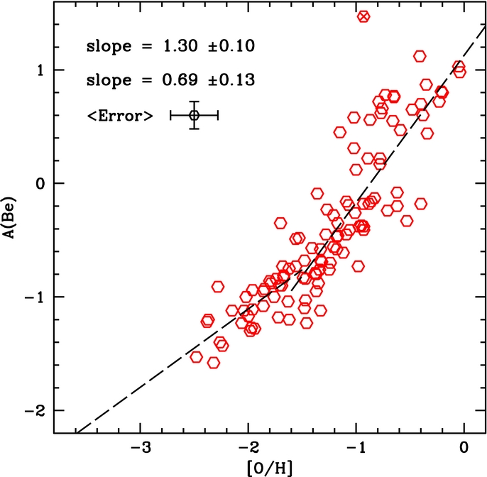
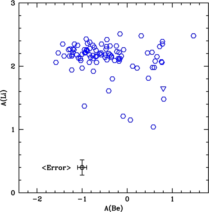
Figure 27. Example of our A(Be) spread analysis for [O/H]. The top panel shows the test for the interval centered at [O/H] = −0.8 with a width of 0.5 dex (gray shaded region). We use the data which is represented by the black filled circles to derive the best fit (solid line) and the prediction interval (dashed lines). The data within the region of interest are the (red) open circles. In this example, 10 out of 30 points lie outside the 95% prediction interval. Based on the binomial theorem, the probability of this occurring by chance is 1.1 × 10⁻⁶. This process is repeated in running steps of 0.01 dex, producing the probability curve shown in the middle panel. For central values of [O/H] between ∼−0.75 and −0.95 (or a range from ∼−0.5 to −1.1), there appears to be a spread in Be at >4σ for a given [O/H]. In the bottom panel, we show the results ignoring the two Be-rich stars HD 106038 and HD 132475 (marked with crosses in the top panel); even in this case the spread appears to be significant.
Download figure:
Standard image High-resolution image
The interval where there is the most spread in Be is between [O/H] = −0.5 and −1.0, which corresponds to −0.9 and −1.6 in [Fe/H].
5. SUMMARY AND CONCLUSIONS
The study of the light elements—Li, Be, and B—is important in advancing our knowledge of cosmology, Galactic evolution, and stellar structure and evolution. We have made observations to determine Be abundances in 117 stars, most of which were obtained from the upgraded HIRES spectrometer on the Keck 10 m telescope. Our spectral resolution is ∼42,000 and our median S/N is 106 per pixel. We have also found abundances of Fe, O, Mg, and Ti. The Be and O abundances were found from spectrum synthesis from the Be ii resonance lines and the OH electronic transitions in the ultraviolet spectral region near 3100 Å. Equivalent widths were measured for Fe i, Fe ii, Ti i, Ti ii, and Mg i lines.
We have determined the stellar parameters spectroscopically from the Fe i lines for Teff and the ionization balance of Ti i and Ti ii or occasionally from Fe i and Fe ii for log g. The value for [Fe/H] comes from the Fe i lines. We have made error estimates from the uncertainties in the stellar parameters for three stars which cover the range in our stellar parameters in Teff, log g, [Fe/H], and ξ.
One of our stars, G 268-32, is a CEMP star according to Aoki et al. (2002). It has [Fe/H] = −2.51. Like BD +44 493, a CEMP star studied by Ito et al. (2009), G 268-32, seems to be devoid of Be and we set an upper limit of A(Be) = −1.5. Although the compilation by Charbonnel & Primas (2005) gives A(Li) = 1.99 for G 268-32 (HIP 3446), when we use our model and Thorburn's (1994) equivalent width for Li, we find A(Li) = 2.32.
We found a linear fit between the [Fe/H] and A(Be) over three orders of magnitude in [Fe/H] with a slope of 0.88 ± 0.03. Although we found no support for the idea of a plateau in Be at low metallicities, we did find that Be is enriched relative to Fe changing from [Be/Fe] near +0.2 at [Fe/H] near −3.3 down to ∼0.0 near [Fe/H] ∼−1.7. This supports the idea that much of the Be was formed by the "supernovae" mechanism in the early history of the Galaxy. The Fe is formed primarily from intermediate-mass stars from SNe Ia.
We examined the relationship between Be and O because they are directly related as the light elements are formed by spallation with CNO atoms. This relationship can also be fit by a straight line with a slope of 1.04 ± 0.05 over two and a half orders of magnitude in [O/H]. There is more scatter in the Be–O data than in the Be–Fe data and the scatter is not uniformly distributed; both the lowest Be points and the highest Be points lie above the best-fit line. We tried fitting the results with two lines dividing the sample at [O/H] = −1.6. The Be-poor and O-poor stars are fitted with a slope of 0.69 ± 0.13, while the Be-rich/O-rich stars have a steeper slope of 1.30 ± 0.10. A change of slope between A(Be) and [O/H] would be expected due to the change in the dominant mechanism of Be formation going from the "supernovae" mechanism to the classical GCR mechanism. It is clear that the change in slope is caused by the Be abundance rather than by the O abundance as indicated by the smaller scatter and clear linear fit between [Fe/H] and [O/H].
The O abundance found from the UV lines of OH is sensitive to both the temperature and the gravity. Therefore, we decided to use the alpha-elements, Ti and Mg, as surrogates for O. We found a remarkably tight correlation between [Ti/H] and [Fe/H] and between [Mg/H] and [Fe/H]. This indicates that our stellar parameters are well determined. The slope between [Mg/H] and [Fe/H] is 0.94 ± 0.01.
We found that A(Be) tracks [Ti/H] very well with a slope of 1.00 ± 0.04 and that A(Be) tracks [Mg/H] very well with a slope of 0.88 ± 0.03. As with the Be versus O relation, both the lowest Be stars and the highest Be stars lie above the linear fit, which may indicate that two slopes would be a better representation of the data.
We have searched the literature for Li abundances in our stars and found results for 96 of our 117 stars. Most of our stars have Li abundances near the observed Li plateau of A(Li) ∼ 2.2. Seven stars were below A(Li) = 1.8. With the possible exception of our coolest star, BD +37° 1458, none of the Li-depleted stars are Be-deficient for their [Fe/H] values. If BD +37° 1458 is depleted in Be it is only a mild depletion. We note that our two stars with enhanced Be, HD 106038 and HD 132475, also have enhanced Li.
Gratton et al. (2003) have established kinematic criteria for distinguishing between a dissipative collapse population (mainly thick disk and halo stars) and an accretive population (mainly halo stars). We have kinematic information on 114 stars and our sample is equally divided between the two groups. Most of our stars have prograde motion, but 33 are on retrograde orbits with V < −220 km s−1. The stars in all three groups cover nearly the full range in both [Fe/H] and [O/H].
The dependence of A(Be) on [Fe/H] and on [O/H] shows distinct differences between the dissipative and the accretive groups. The dissipative stars have a steeper slope of A(Be) with both [Fe/H] and [O/H] than the accretive and retrograde stars. For the Be relationship with [Fe/H] the slope for the accretive stars is 0.68 ± 0.04 and for the dissipative stars is 0.94 ± 0.04. The slopes of A(Be) with respect to [O/H] are both steeper than with [Fe/H]: 0.76 ± 0.06 for the accretive stars and 1.13 ± 0.08 for the dissipative stars. The Be in the accretive stars may have been created in the vicinity of SN II stars in the early days of the Galaxy formation and accretion of small stellar systems. The Be in the dissipative stars may have been formed preferentially by GCR spallation reactions.
We have found that there are no stars in the accretive and retrograde groups with A(Be) > 0.35, except for the two stars with enhanced Be. Those two stars are thought to have originated in the vicinity of a hypernova or in entrained superbubbles with multiple SNe (Boesgaard & Novicki 2006; Smiljanic et al. 2009). In general, the accretive and retrograde stars were not formed in an environment rich in Be.
The distribution of [Be/Fe] with the rest-frame velocity is flat for the accretive and retrograde stars with the mean over the range of 400 km s−1 near [Be/Fe] = 0.0. The dissipative stars have higher [Be/Fe] at low values of vRF.
It was suggested by Suzuki & Yoshii (2001) and Pasquini et al. (2005) and then further explored by Smiljanic et al. (2009) that the stellar abundance of Be can be used as a chronometer. In our large sample of 116 stars we find that Be is not as good as Fe as a chronometer. In the usual plot of [O/Fe] versus A(Be), there is more scatter in the data than in the plot of [O/Fe] versus [Fe/H]. The Be abundance is less well determined than the Fe abundance. If we divide the stars into the dissipative and accretive (and retrograde) subgroups, the fit to the data is no different from the fit with the full sample. For all plots there is more scatter in A(Be) for data with A(Be) > 0.0 and with [Fe/H] > −1.4, i.e., for the more recently formed stars.
Related to the use of Be as a chronometer is the issue of whether there is a spread in Be at a given metallicity, as measured by Fe, O, Ti, and Mg. There is empirical evidence for a spread through comparisons of Be in pairs of stars with the same stellar parameters. Smiljanic et al. (2009) show four such pairs. Boesgaard et al. (2010) have done statistical tests which show a real dispersion in A(Be) at a given [O/H] at the 4σ level and at a given [Fe/H] at the 3σ level. With a similar analysis done here with the larger sample, we find more support for the reality of the spread in A(Be) with [O/H]. There is evidence at the 4σ level for a spread in A(Be) at [O/H] from −0.5 to −1.0, which corresponds to [Fe/H] = −0.9 to −1.6.
We are grateful to the various support astronomers and observing assistants who helped us over the many observing runs for this project. We are indebted to Hai Fu for his IRAF modification that enabled us to measure equivalent widths quickly and easily. We thank Gabriel Dima for determining Li abundances in six of our stars. We acknowledge support from NSF through grant AST 05-05899 to A.M.B.
APPENDIX
Table 6 gives the measured equivalent widths for the stars in this paper by the code numbers given in Table 1. Table 7 gives the measured equivalent widths for the Mg i lines for the stars in Rich & Boesgaard (2009) according to the code numbers in Table 1 in that paper.
Table 6. Measured Equivalent Widths
| λ (Å) | Ele. | 1 | 2 | 3 | 4 | 5 | 6 | 7 | 8 | 9 | 10 | 11 | 12 |
|---|---|---|---|---|---|---|---|---|---|---|---|---|---|
| 3100.304 | Fe i | ... | ... | ... | ... | ... | ... | ... | ... | ... | ... | ... | ... |
| 3100.665 | Fe i | ... | ... | ... | ... | ... | ... | ... | ... | ... | ... | ... | ... |
| 3100.836 | Fe i | 10.0 | ... | ... | ... | ... | ... | ... | 17.0 | ... | 16.0 | ... | ... |
| 3116.631 | Fe i | 51.2 | 29.9 | 47.4 | ... | 33.6 | ... | ... | ... | ... | ... | 29.99 | ... |
| 3129.334 | Fe i | 26.7 | 11.1 | 14.9 | 36.03 | 11.0 | ... | ... | ... | 41.7 | 28.1 | 11.96 | ... |
| 3132.519 | Fe i | 12.0 | 10.4 | ... | 22.91 | 6.7 | ... | ... | ... | 24.8 | ... | ... | ... |
| 3142.454 | Fe i | ... | ... | ... | ... | ... | ... | ... | ... | ... | 35.3 | ... | ... |
| 3142.889 | Fe i | 17.3 | 13.0 | 13.1 | ... | ... | ... | ... | ... | 32.3 | 21.1 | 9.67 | ... |
| 3143.984 | Fe i | ... | ... | ... | ... | ... | ... | ... | ... | ... | ... | ... | ... |
| 4494.563 | Fe i | 37.3 | 19.3 | 36.4 | 51.24 | 27.6 | ... | ... | 54.6 | 60.1 | 56.6 | 19.35 | ... |
Only a portion of this table is shown here to demonstrate its form and content. A machine-readable version of the full table is available.
Download table as: DataTypeset image
Table 7. Measured Equivalent Widths
| λ (Å) | Ele. | 1 | 2 | 3 | 4 | 5 | 6 | 7 | 8 | 9 | 10 | 11 | 12 |
|---|---|---|---|---|---|---|---|---|---|---|---|---|---|
| 4571.099 | Mg i | ... | 6.4 | ... | ... | 9.4 | ... | ... | ... | ... | 5.4 | ... | ... |
| 4702.998 | Mg i | 25.5 | 54.7 | 19.44 | 19.9 | 45.1 | 40.4 | 27.6 | 21.8 | 20.3 | 32.9 | 25.4 | 30.8 |
| 4730.033 | Mg i | ... | ... | ... | ... | ... | ... | ... | ... | ... | ... | ... | ... |
| λ (Å) | Ele. | 13 | 14 | 15 | 16 | 17 | 18 | 19 | 20 | 21 | 22 | 23 | |
| 4571.099 | Mg i | 10.1 | 8.4 | ... | ... | ... | ... | 11.1 | ... | 5.3 | ... | ... | |
| 4702.998 | Mg i | 63.1 | 44.3 | 10.6 | 37.1 | 22.4 | 19.5 | 62.0 | 23.2 | 33.3 | 15.2 | 10.4 | |
| 4730.033 | Mg i | ... | ... | ... | ... | ... | ... | ... | ... | ... | ... | ... | |
Download table as: ASCIITypeset image
Footnotes
- 3
- 4
IRAF is distributed by the National Optical Astronomy Observatory, which is operated by the Association of Universities for Research in Astronomy, Inc., under cooperative agreement with the National Science Foundation.
- 5