


ABSTRACT
The convective flow in the moments preceding the explosion of a Type Ia supernova determines where the initial flames that subsequently burn through the star first ignite. We continue our exploration of the final hours of this convection using the low Mach number hydrodynamics code, MAESTRO. We present calculations exploring the effects of slow rotation and show diagnostics that examine the distribution of likely ignition points. In the current calculations, we see a well-defined convection region persist up to the point of ignition, and we see that even a little rotation is enough to break the coherence of the convective flow seen in the radial velocity field. Our results suggest that off-center ignition may be favored, with ignition ranging out to a radius of 100 km and a maximum likelihood of ignition at a radius around 50 km.
Export citation and abstract BibTeX RIS
1. INTRODUCTION
The most widely investigated model for a Type Ia supernova (SN Ia) involves a white dwarf accreting from a companion and nearing the Chandrasekhar mass (the "single-degenerate" scenario; see Hillebrandt & Niemeyer 2000 for a review). As the white dwarf approaches this limit, the temperature near the center is high enough that carbon fusion reactions begin, heating the interior and driving convection throughout the white dwarf. This convective phase can last for centuries (Woosley et al. 2004). Eventually, the temperature is hot enough that the reactions proceed faster than the fluid can cool via expansion, and a flame front is born (Nomoto et al. 1984). This flame then propagates through the star in seconds, possibly transitioning into a detonation. The energy released from the reactions overcomes the gravitational binding energy of the star, resulting in the explosion. This model has generally been successful in explaining observations, including stratification of the ash composition (Gamezo et al. 2005) and light curves and spectra (Woosley et al. 2007; Röpke et al. 2007a; Kasen et al. 2008).
Alternate progenitor scenarios exist, including merging white dwarfs. Here, the interaction between the stars leads to the disruption of the less massive star, and may result in the formation of a hot envelope and the subsequent accretion of mass by the remaining white dwarf (Yoon et al. 2007; Motl et al. 2007; Lorén-Aguilar et al. 2009). A potential problem with this picture is that the carbon may ignite when the stars first come in contact, leading to a collapse to a neutron star (Nomoto & Kondo 1991). If this can be avoided, the merger remnant may look very similar to a progenitor in the single-degenerate picture just before ignition. This suggests that some of what we learn about the convective flow in our calculations of ignition in the single-degenerate scenario may carry over to a massive white dwarf formed from a merger.
A final, alternate progenitor scenario is the ignition of a burning front in the accreted helium layer on a sub-Chandrasekhar-mass white dwarf. If a detonation can begin in a thin helium layer and propagate into the underlying carbon/oxygen white dwarf, the result may resemble a (faint) SN Ia (Sim et al. 2010; Shen et al. 2010; Woosley & Kasen 2011). While the calculations presented here do not address this last model, the low Mach number simulation technique we describe here is directly applicable to modeling ignition in an accreted helium layer, and we will address this problem in the near future.
In this paper, we continue our exploration of the convection in the single-degenerate scenario, leading right up to the ignition of the first flame. In this picture, the location and number of the first flames to ignite can have a large effect on the subsequent explosion outcome (Niemeyer et al. 1996; Plewa et al. 2004; Livne et al. 2005; García-Senz & Bravo 2005). Improving explosion models requires better initial conditions, and hence modeling the convective period preceding ignition. Early studies of this convective period cut out the very center of the star and modeled only a two-dimensional wedge (Höflich & Stein 2002; Stein & Wheeler 2006), finding ignition near the center as the flow converged in the wedge geometry. Three-dimensional anelastic calculations by Kuhlen et al. (2006) modeled the inner 500 km of the convective region (cutting out the very center of the star) and found a large-scale dipole flow dominates. Neither of these studies included the very center of the star, and therefore did not allow the fluid to flow through the center.
Accreting white dwarfs gain angular momentum and are expected to rotate (see, for example, Yoon & Langer 2004). The centrifugal force in a rotating white dwarf counteracts gravity, increasing the maximum mass of a white dwarf. It may be possible that rapidly rotating white dwarfs can explain observed super-Chandrasekhar SNe Ia events (Pfannes et al. 2010). Slow rotation was shown to affect the convective flow in the calculations of Kuhlen et al. (2006).
In this paper, we explore the effect of rotation on the large-scale convective flow and examine where the ignition is most likely to take place. Our approach models the entire white dwarf, and we restrict ourselves to low rotation rates to minimize the deviation from sphericity. Our simulations use the MAESTRO algorithm, which was developed and tested in a series of papers (Almgren et al. 2006a, 2006b, 2008), and has been shown to allow for the efficient simulation of highly subsonic flows. This work builds off of our previous study (Zingale et al. 2009, henceforth Paper IV) where we demonstrated the ability of MAESTRO to accurately model convection in a white dwarf over long timescales. The simulations in this paper use a recently updated version of the MAESTRO algorithm (Nonaka et al. 2010, henceforth Paper V). In Section 2, we discuss the numerical method, focusing on the improvements since Paper IV. In Section 3, we present the results of several calculations leading up to ignition. Finally, in Section 4, we summarize and conclude.
2. NUMERICAL METHODOLOGY AND SETUP
In the low Mach number formulation, the equations of hydrodynamics are reformulated to analytically filter sound waves from the system, while retaining the local compressibility effects due to heat release and the expansion/contraction of a fluid element as it moves in a stratified atmosphere (Almgren et al. 2006a). In our formulation, the fluid state is described in terms of the full state as well as the one-dimensional hydrostatic base state (characterized by a density, ρ0, and pressure, p0, with  , where g is the gravitational acceleration and
  is the unit vector in the radial direction). In parts of the algorithm we work with perturbational quantities, defined as the deviation of the full state from the base state. The primary condition for the validity of the model is that the deviation of the full pressure from the base state pressure remain small.
As reactions heat the stellar core, the star expands. We capture this expansion by allowing the net heating to define a one-dimensional base state velocity, w0, that is used to evolve the base state in time. The base state velocity satisfies  , where the overline notation indicates the lateral average over a layer of constant radius and
  is the full velocity field. The local velocity,
  , satisfies the constraint,

where β0 is a density-like variable that captures the expansion of a fluid element due to changing radius, S represents local changes to compressibility due to heat release and compositional mixing. See Paper V for the derivation and details of base state evolution for a spherical, self-gravitating star. When the magnitude of the heating is significant, capturing the expansion of the base state is critical to maintaining the validity of the algorithm over long timescales. This was demonstrated for plane-parallel atmospheres in Almgren et al. (2006b).
There have been a number of changes both to the algorithm and the input physics compared to Paper IV. We use the version of the algorithm as detailed in Paper V. Briefly, the changes from Paper IV are as follows.
- 1.Base state evolution. We now evolve the hydrostatic base state in response to the large-scale heating. We argued in Paper IV that the expected expansion is small. Here, we include it now for completeness and show the amount of expansion in Section 3.1.
- 2.Better averaging/interpolation. The coupling between the one-dimensional radial base state and the three-dimensional Cartesian state is greatly improved. This better coupling provides greater accuracy in all parts of the algorithm where the base state and full state interact with each other, and is especially important for the expanding base state. As with Paper IV, we continue to set the radial base state spacing, Δr to be 1/5th of the Cartesian grid spacing, Δx.
- 3.
- 4.New initial model. In order to reduce the additional computational time which would be necessary to reach ignition with the new, slightly weaker energetics, we start the calculations with a slightly hotter initial model (central temperature of 6.25 × 10⁸ K instead of 6 × 10⁸ K). We also change the amplitude of the initial velocity perturbation. The details of these changes are described in Section 2.2.
- 5.
- 6.Lower cutoff density/new sponge. We have lowered the low-density cutoff (ρcutoff) from 106 g cm−3 to 105 g cm−3 and adjusted the sponge term in the momentum equation. In effect, this means that we are modeling more of the outer region of the star than in Paper IV. This is described in Section 2.3.
- 7.Rotation. We now include the forcing that describes a rotating star. This is described in Section 2.4.
- 8.Diagnostics. We have enhanced the runtime diagnostics, keeping more detailed information about the fluid state at each time step. We now track the spatial location of the hot spot (i.e., the hottest point) in the convective zone at each time step.
In the next subsections, we discuss the microphysics, initial model, sponging, and rotation terms.
2.1. Microphysics
We again use the public version of the general stellar equation of state described in Timmes & Swesty (2000) and Fryxell et al. (2000) to describe the state of the fluid. This has contributions from ions, electrons, and radiation, and includes Coulomb corrections.
We have improved the energetics from carbon burning by incorporating the results of Chamulak et al. (2008). Chamulak et al. (2008) show that one can capture the effects of a larger network by using a simple multiplier on the 12C + 12C reaction rate, and adjusting the energy release. We use the numbers provided in Chamulak et al. (2008) and fit a parabola to the tabulated energy release values provided. Again, we use the reaction rate provided in Caughlan & Fowler (1988) and screening as described in Graboske et al. (1973), Weaver et al. (1978), Alastuey & Jancovici (1978), and Itoh et al. (1979). For the ash composition, we take a mix of the ash state described in Chamulak et al. (2008), assuming that electron captures onto 23Ne have frozen out, giving an average atomic weight of the ash of A = 18 and an average atomic number of the ash of Z = 8.8. The overall effect of this change is a slightly lower energy generation rate, but the overall dynamics evolve very similarly to that of Zingale et al. (2009). Finally, we note that, as discussed in Almgren et al. (2008), when integrating the reaction network we evolve a temperature equation for the sole purpose of evaluating the reaction rates. To reduce the computational demands, we freeze the specific heat, cp, at the start of the integration. Our simulations show that even up to the point of ignition, cp changes by <1% in the center or hot spot per time step, demonstrating that this approximation is valid. The final temperature is based on the energy release from the reactions and not the integrated temperature.
2.2. Initial Model
We start with a slightly hotter initial model than before—the central temperature at the time of mapping onto the Cartesian grid is 6.25 × 10⁸ K instead of the 6 × 10⁸ K from Paper IV. This allows us to reduce the increase in computational time to reach ignition that would result from the fact that the new reaction energetics have lower energy release. The temperature and density structure of the initial model is shown in Figure 1. As with Paper IV, the model is characterized by an inner convectively unstable region and an outer stable region. The convective region encompasses the inner 1.156 M☉ of the star. The total mass of the star is 1.383 M☉. In adapting the one-dimensional initial model to our code, we grouped all of the "ash" material (anything other than 12C or 16O) into the ash state used by our network. The initial model is then put into hydrostatic equilibrium on our radial grid with the equation of state using the techniques discussed in Zingale et al. (2002). As in Paper IV, we constrain the entropy in the convective region to be constant initially. This represents a small thermodynamic adjustment.
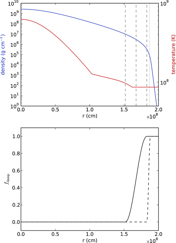
Figure 1. White dwarf initial model and sponge parameters. The top panel shows the initial white dwarf density (blue line) and temperature (red line). The vertical dashed lines mark the location of the start, middle, and top of the inner sponge. The dotted line marks the location of ρcutoff. The bottom panel shows the damping function for the inner sponge (solid line) and outer sponge (dashed line).
Download figure:
Standard image High-resolution imageAt t = 0, reactions at the center of the star generate heat that begins to drive convection. In the absence of an initially non-zero convective velocity field, the center of the star will runaway prematurely. In order to begin the calculation sensibly, as in Paper IV we perturb the initial velocity field to try to carry away some of the heat. The form of the velocity perturbation is unchanged from Paper IV, and consists of 27 Fourier components with random phases and amplitudes. The perturbation is described by an amplitude, A, a characteristic perturbation scale, σ, a characteristic region to apply the perturbation defined by rpert, and a transition thickness between the perturbed and unperturbed region, d. We leave σ, rpert, and d unchanged from Paper IV with values of 107 cm, 2 × 107 cm, and 105 cm, respectively.
Even with the velocity perturbation, the temperature at the center of the star spikes initially, until a large-scale convective flow develops and redistributes the heat. We found that increasing the velocity perturbation amplitude, A, reduces the amount by which the temperature spikes (see Figure 2). Based on this behavior, we change the amplitude of the perturbation used in the main calculations here from 105 cm s−1 in Paper IV to 106 cm s−1 without affecting the long-time behavior of the system.

Figure 2. Peak temperature vs. time for the early evolution of a 2563 convecting white dwarf, with three different values for the initial velocity perturbation amplitude, A. We see that the higher the value of the initial velocity perturbation, the smaller in amplitude the early spike in peak temperature. After this transient spike, the trends in peak temperature for all three values of A match well.
Download figure:
Standard image High-resolution image2.3. Cutoff Densities and Sponging
Imposing the divergence constraint on the velocity field (Equation (1)) at the edge of the star generates large velocities if we allow the density to drop to arbitrarily small values outside the star. This is basically a statement of conservation of momentum—as the density drops the velocity correspondingly increases. We combat this in two ways. First, we modify the behavior of the algorithm in regions where the density falls below prescribed density cutoffs. Second, we add a forcing term to the momentum equation (a sponge) that forces the velocities outside the star toward zero. Both of these were described in Paper IV. Here, we discuss the values of these quantities used for the present calculations.
As described in Paper IV, we define a low-density cutoff, ρcutoff, below which we keep the density from the initial model fixed. This prevents the velocities at the edge of the star from growing too large as a result of the divergence constraint. In Paper IV, we used ρcutoff = 106 g cm−3. Experiments with the expanding base state showed that we more accurately capture the expansion with a lower value for the density cutoff. For the present runs, we set ρcutoff = 105 g cm−3. The mass of the star contained within this cutoff is 1.383 M☉—essentially the entire star. The location of the cutoff density in our initial model is indicated as the dotted vertical line in the top panel of Figure 1. The lower value of ρcutoff used here, compared to Paper IV, means that more of the stably stratified region is modeled on the grid. Figure 3 shows a one-dimensional base state expansion calculation with three different choices of ρcutoff. We see that our choice of ρcutoff = 105 g cm−3 matches the solution for ρcutoff = 10−4 g cm−3 well, indicating that this choice of ρcutoff reasonably captures the expansion of the star.
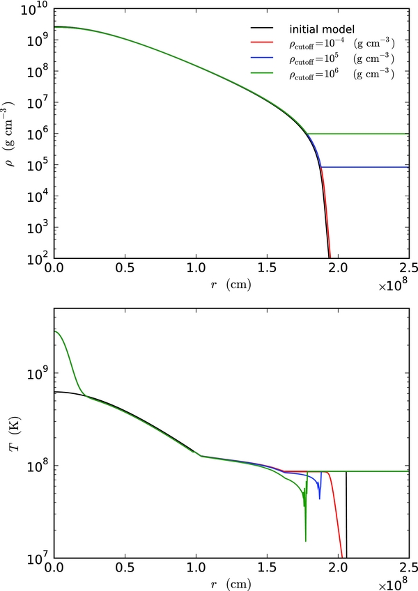
Figure 3. One-dimensional test problem where we heat the interior of the white dwarf for 5 s and watch the resulting hydrostatic readjustment. Three different values of ρcutoff were used. We see that the run with ρcutoff = 105 g cm−3 (the value used for the main simulations presented here) agrees well with the run using ρcutoff = 10−4 g cm−3.
Download figure:
Standard image High-resolution imageAlthough lowering ρcutoff from that used in Paper IV to the present value captures the expansion of the base state well, it results in an increase in the velocities near the edge of the star. To compensate for this, we exclude the buoyancy term and centrifugal force (see Section 2.4) from the velocity evolution equation in regions where the density is less than 5 ρcutoff.
To help control the magnitude of the velocities at the edge of the star, we also use sponging terms in the velocity evolution equation. These work to force the velocities toward zero outside the star. We carry two sponges, an inner sponge that works at the very edge of the white dwarf, and an outer sponge which is in effect outside of the star. We define the start, center, and top radius of the inner sponge in terms of density. Equivalently, the radius corresponding to the start, center, and top can be found by inverting the base state density profile, ρ0(r, t), which we write as r0(ρ, t). In the present paper, we decouple the location of each sponge from the value of ρcutoff. We define a density at which to center the sponge, ρmd, and apply a multiplicative factor, fsp, to mark the start of the sponge. For the present calculations, we take ρmd = 3 × 10⁶ g cm−3 and fsp = 3.333 for the inner sponge. In terms of radius, the sponge turns on at rsp = r0(fsp ρmd). The top of the sponge (where the sponge is in full effect) is then rtp = 2r0(ρmd) − rsp. The functional form of the sponge is unchanged from Paper IV. The mass contained within the radius corresponding to the inner sponge starting density (fspρmd) is 1.363 M☉. The center of the inner sponge is keyed to the same density, ρmd, as in Paper IV, but the transition region is now much tighter. Finally, we retain a second sponge outside of the star (the outer sponge), as defined in Paper IV, but we now start it just outside the region where the inner sponge turns fully on. The bottom panel of Figure 1 shows the profiles of the inner and outer sponge damping functions together with the initial model. Also shown in the top panel as dashed vertical lines are the location of the starting, center, and top radii of the inner sponge. We explored the sensitivity of the results to the choice of ρcutoff (and sponge location) in Paper IV. The values adopted here are within the range explored there.
Finally, as in Papers IV and V, we define an anelastic cutoff density, ρanelastic, in order to suppress spurious wave formation at the outer boundary of the star. For radial locations where ρ0 ⩽ ρanelastic, we modify the computation of β0, i.e., we compute β0 using β0(ρ0) = (ρ0/ρanelastic)β0(ρanelastic). We set ρanelastic = 106 g cm−3, the lower of the two values explored in Paper IV. The mass enclosed in the radius corresponding to this density is 1.382 M☉.
2.4. Rotation
To incorporate rotation into our equation set, we add the Coriolis and centrifugal terms to the velocity evolution equation (see, for example, Tritton 1988). We take the rotation to be uniform, with the axis aligned with the z-coordinate. In this case, it can be described by an angular velocity,  . The velocity equation becomes
where π is the dynamic pressure (see Almgren et al. 2008 for a derivation of the velocity equation). The Cartesian components of the Coriolis term are
where u and v are the x- and y-components of  , respectively. The Cartesian components of the centrifugal term are
We note that Kuhlen et al. (2006) did not include the centrifugal term, arguing that the Coriolis term dominates.
We also include these terms in the evolution equation for the local velocity field,  ,
,
where π0 is the analogous base state dynamic pressure (see Almgren et al. 2008 for details). When predicting the time-centered advective velocities,  (Steps 3 and 7 in Paper V), we use the velocity field at the old time level,
  , together with the base state velocity to evaluate the Coriolis force. In the final velocity update (Step 11 in Paper V), we use the time-centered
  velocities together with the base state velocity in the Coriolis force to maintain second-order accuracy. Note that no forcing is explicitly included in the evolution equation for w0.
We define the base state as a function of radius and time only; implicit in this is an assumption that the hydrostatic star is approximately spherically symmetric. Very rapid rotation will distort even the unperturbed star, making the current assumption invalid. Therefore, in the present study, we restrict ourselves to small rotation rates. Since the rotation rates are small, we do not include an angle-averaged centrifugal force term in the definition of the base state hydrostatic equilibrium.
2.5. Diagnostics
We retain many of the same global diagnostics described in Paper IV. We define the region of interest for our calculations to be the region enclosed by the radius at which the inner sponge starts (ρ > fspρmd). Unless otherwise noted, all global quantities will exclude the region of the star where the density is less than the density at which the inner sponge is turned on. In addition to the peak temperature as a function of time, detailed in Paper IV, we now also store the coordinate location and velocity of the zone with the peak temperature. This allows us to examine the radius of potential ignitions as a function of time.
3. RESULTS
In all, we present five different calculations (labeled A–E for convenience). The highest resolution calculation (simulation A) is a 5763 non-rotating model. This corresponds to an 8.7 km resolution. To explore the effects of rotation, two 3843 runs were done (corresponding to a 13 km resolution—the same as in Paper IV). Simulation B is with no rotation and simulation C has a rotation rate of 1.5% of the Keplerian frequency at the outer edge of the star. This corresponds to Ω = 0.084 s−1. Finally, two low-resolution (2563 zones; 19.5 km resolution) calculations were run to assess the robustness of features observed in the main calculation. Simulation D is non-rotating and simulation E is rotating at 1.5% of the Keplerian rate. Table 1 summarizes the results from these calculations, as well as the results from Paper IV for comparison. We report the radius of the ignition point, Rignite, and the outward radial velocity at the ignition point, (vr)ignite. We define ignition as the time when the maximum temperature reaches 8 × 10⁸ K.
Table 1. Ignition Parameters from Different Simulations
| ID | Simulation Description | Grid | Δx | Rignite | (vr)ignitea | Source |
|---|---|---|---|---|---|---|
| (km) | (km) | ( km s−1) | ||||
| A | Non-rotating WD, Tc = 6.25 × 10⁸ K initial model, new energetics, PPM, ρcutoff = 105 g cm−3 | 5763 | 8.7 | 25.7 | 5.1 | This paper |
| B | Non-rotating WD, Tc = 6.25 × 10⁸ K initial model, new energetics, PPM, ρcutoff = 105 g cm−3 | 3843 | 13.0 | 11.3 | 0.14 | This paper |
| C | Rotating WD (1.5% Keplerian), Tc = 6.25 × 10⁸ K initial model, new energetics, PPM, ρcutoff = 105 g cm−3 | 3843 | 13.0 | 46.4 | 7.0 | This paper |
| D | Non-rotating WD, Tc = 6.25 × 10⁸ K initial model, new energetics, PPM, ρcutoff = 105 g cm−3 | 2563 | 19.5 | 57.8 | 48.3 | This paper |
| E | Rotating WD (1.5% Keplerian), Tc = 6.25 × 10⁸ K initial model, new energetics, PPM, ρcutoff = 105 g cm−3 | 2563 | 19.5 | 42.6 | 13.2 | This paper |
| - | Non-rotating WD, Tc = 6 × 10⁸ K initial model, old energetics, piecewise linear, ρcutoff = 106 g cm−3 | 2563 | 19.5 | 32.4 | 2.9 | Zingale et al. (2009) |
| - | Non-rotating WD, Tc = 6 × 10⁸ K initial model, old energetics, piecewise linear, ρcutoff = 3 × 10⁶ g cm−3 | 2563 | 19.5 | 84.6 | 39.0 | Zingale et al. (2009) |
| - | Non-rotating WD, Tc = 6 × 10⁸ K initial model, old energetics, piecewise linear, ρcutoff = 3 × 10⁶ g cm−3 | 3843 | 13.0 | 21.6 | 4.8 | Zingale et al. (2009) |
Note. aPositive values indicate outflow, negative values indicate inflow.
Download table as: ASCIITypeset image
We note that we tried a run with a rotation rate corresponding to 3% of the Keplerian rate. After the initial rise in temperature we expected when the convective velocity field has not yet developed to carry away the energy generated at the center, the temperature began to steadily decrease, likely because the star was adjusting to the new hydrostatic balance. While this is likely a transient behavior, we did not have the computational resources to pursue this further.
3.1. General Behavior
Figure 4 shows the peak temperature as a function of time for simulation A (5763, non-rotating), and Figure 5 shows the two 3843 calculations (B and C). The general behavior is similar to that shown in Paper IV, with the ignition following rapidly after the peak temperature crosses 7 × 10⁸ K. We note that the rotating case reaches ignition much earlier than the non-rotating case. We see the same behavior in the lower resolution, 2563, calculations (D and E), with the rotating model igniting well before the non-rotating case (see Figure 6). This suggests that this may be a general trend. We also note that, as in Paper IV, the lower resolution runs ignite sooner than the higher resolution runs.
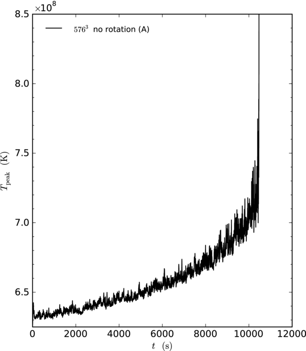
Figure 4. Peak temperature in the region ρ > fspρmd for the non-rotating 5763 simulation of the convecting white dwarf (simulation A).
Download figure:
Standard image High-resolution image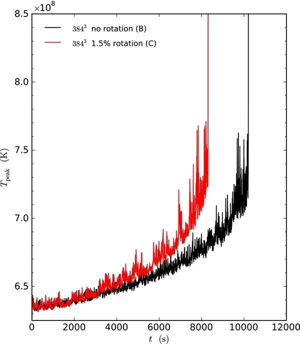
Figure 5. Peak temperature in the region ρ > fspρmd for both the non-rotating and rotating 3843 simulations of the convecting white dwarf (simulations B and C).
Download figure:
Standard image High-resolution image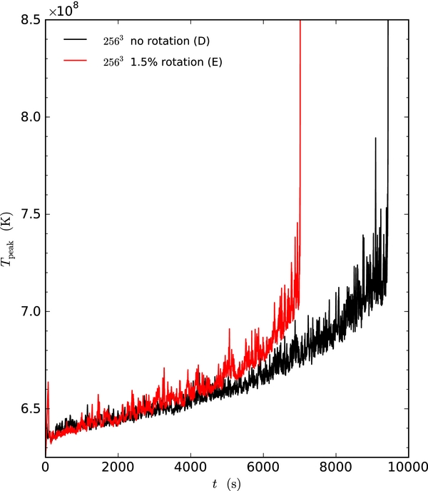
Figure 6. Peak temperature in the region ρ > fspρmd for both the non-rotating and rotating 2563 simulations of the convecting white dwarf (simulations D and E).
Download figure:
Standard image High-resolution imageFigure 7 shows the peak radial velocity for simulation A, and Figure 8 shows the peak radial velocity in the region of interest for simulations B and C. The overall behavior is very similar to that of Paper IV—the peak radial velocity ∼107 cm s−1 for most of the evolution with a rise at late times. We note that the rotating calculation shows many large-amplitude fluctuations away from this general trend throughout the calculation. In the non-rotating case, these departures are much lower in amplitude. The peak Mach number in the convective region as a function of time for simulation A and simulations B and C is shown in Figures 9 and 10. Again, we see behavior similar to that of Paper IV, with the Mach number staying around 0.05 until we are close to ignition.
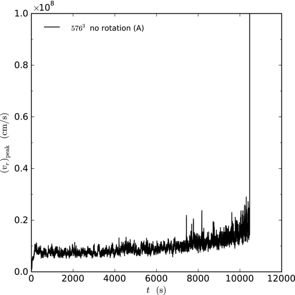
Figure 7. Peak radial velocity in the region ρ > fspρmd for the non-rotating 5763 simulation of the convecting white dwarf (simulation A).
Download figure:
Standard image High-resolution image
Figure 8. Comparison of the peak radial velocity in the region ρ > fspρmd for both the non-rotating and rotating 3843 simulation of the convecting white dwarf (simulations B and C).
Download figure:
Standard image High-resolution image
Figure 9. Peak Mach number in the region ρ > fspρmd for the non-rotating 5763 simulation of the convecting white dwarf (simulation A).
Download figure:
Standard image High-resolution image
Figure 10. Comparison of the peak Mach number in the region ρ > fspρmd for both the non-rotating and rotating 3843 simulation of the convecting white dwarf (simulations B and C).
Download figure:
Standard image High-resolution imageFigure 11 shows the vorticity ( ) around the time of ignition for simulations A through C. In contrast to the calculations presented in Paper IV, the present calculations maintain a sharp boundary between the convectively unstable interior and the stably stratified outer portion of the star (about halfway in radius in the star). Unfortunately, we do not know precisely which of the algorithmic changes from Paper IV described earlier have led to the new behavior, and we do not have the computer time to explore each change independently.
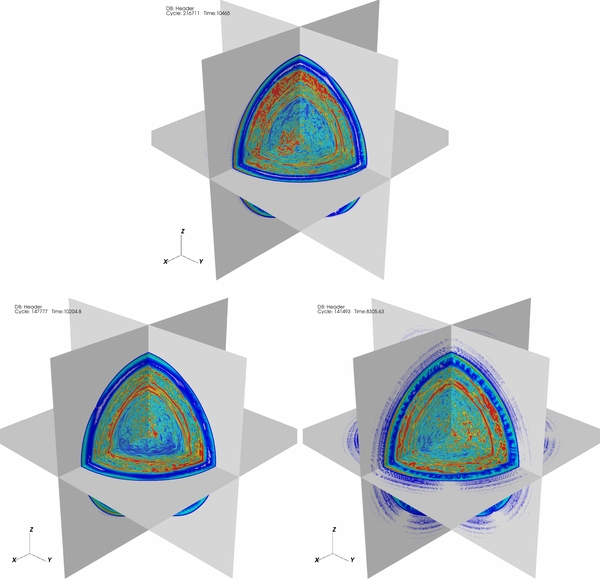
Figure 11. Vorticity in three orthogonal slice planes around the time of ignition for simulations A (top), B (bottom left), and C (bottom right). A clear separation is seen between the convectively unstable interior and the stably stratified outer region about halfway in radius from the center of the star.
Download figure:
Standard image High-resolution imageFigure 12 shows the energy generation rate and radial velocity in the inner portion of the white dwarf for simulation A, less than 1 s before ignition. As it shows, the energy generation is strongly peaked near the center of the star. To get a feel for the qualitative difference in the convective flow for the rotating versus non-rotating cases, Figures 13 and 14 show a time sequence of the inner 1000 km3 of the white dwarf from the start of the simulation up to the point of ignition for simulations B and C. Both the radial velocity and nuclear energy generation rate contours are shown. In both of the panels, it is clear how steeply the energy generation increases toward the center. One can also see that the size of the energy-generating region grows in radius with time, as the center of the star heats up. The outward-flowing radial velocity shows a more coherent behavior in the non-rotating case, appearing as a dipole in many frames, as discussed in Paper IV and in Kuhlen et al. (2006). It is clear that the direction of the dipole changes, and at times, it seems to breakdown. In contrast, the rotating case never shows the same level of coherence in the outward-flowing radial velocity. It seems that even the small amount of rotation modeled here is enough to break the dipole. At times, in the rotating case, flows appear to be in line with the rotation axis. The final frame in each figure is from within 1 s of the point when the peak temperature crosses 8 × 10⁸ K, at which time we say we have ignited. We will continue to explore the behavior of the flow to see if this qualitative behavior holds at higher resolution in future calculations.
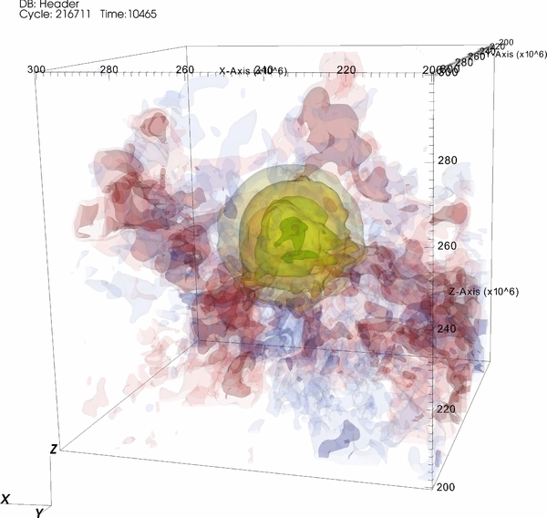
Figure 12. Contours of nuclear energy generation rate (yellow to green to purple, corresponding to 3.16 × 10¹², 1013, 3.16 × 10¹³, 1014, and 3.16 × 10¹⁴ erg g−1 s−1) and radial velocity (red is outflow, corresponding to 2 × 10⁶ and 4 × 106 cm s−1; blue is inflow, corresponding to −2 × 10⁶ and −4 × 106 cm s−1) for the non-rotating 5763 simulation (A), less than 1 s before ignition. Only the inner (1000 km)3 are shown. We see that the energy generation is strongly peaked toward the center.
Download figure:
Standard image High-resolution image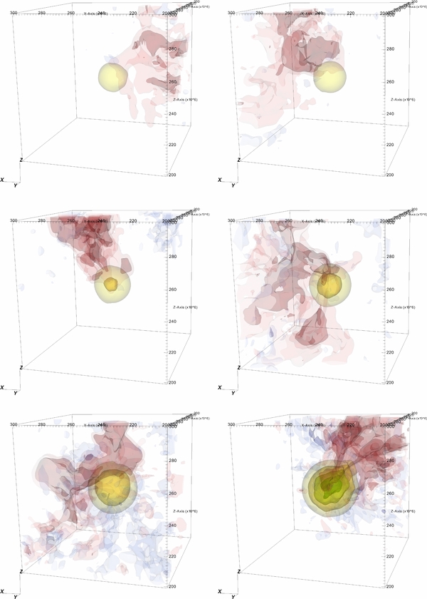
Figure 13. Contours of nuclear energy generation rate (yellow to green to purple, corresponding to 3.16 × 10¹², 1013, 3.16 × 10¹³, 1014, and 3.16 × 10¹⁴ erg g−1 s−1) and radial velocity (red is outflow, corresponding to 2 × 10⁶ and 4 × 106 cm s−1; blue is inflow, corresponding to −2 × 10⁶ and −4 × 106 cm s−1) for the non-rotating run (simulation B). Only the inner (1000 km)3 are shown. Times shown, left to right, top to bottom are 1000 s, 3000 s, 5000 s, 7000 s, 9000 s, and 10204.8 s. This last time corresponds to just under 0.2 s before the peak temperature crossed 8 × 10⁸ K.
Download figure:
Standard image High-resolution image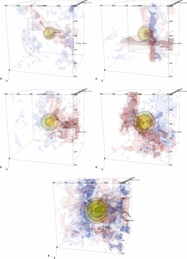
Figure 14. Contours of nuclear energy generation rate (yellow to green to purple, corresponding to 3.16 × 10¹², 1013, 3.16 × 10¹³, 1014, and 3.16 × 10¹⁴ erg g−1 s−1) and radial velocity (red is outflow, corresponding to 2 × 10⁶ and 4 × 106 cm s−1; blue is inflow, corresponding to −2 × 10⁶ and −4 × 106 cm s−1) for the rotating run (simulation C). Only the inner (1000 km)3 are shown. Times shown, left to right, top to bottom, are 1000 s, 3000 s, 5000 s, 7000 s, and 8305.6 s. This last time corresponds to just under 1 s after the peak temperature crossed 8 × 10⁸ K.
Download figure:
Standard image High-resolution imageFigure 15 shows the temperature and density deviations from the base state in three orthogonal slice planes in a 963 zone volume centered on the star for simulation A ∼1 s before ignition. The black lines mark the center of the domain in each coordinate direction. The overall amplitudes of the deviations from the base state is small.
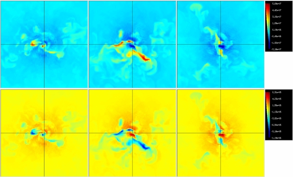
Figure 15. Temperature (top) and density (bottom) deviations from the background state in the inner 963 zones for simulation A ∼ 1 s before ignition. The black lines show the center of the domain in each coordinate direction.
Download figure:
Standard image High-resolution imageFinally, we can look at how much expansion took place by looking at the change in base state density, ρ0, over the course of the calculation. Figure 16 shows ρ0 at the start and end of simulation A, and the relative change over this time. We see that there is a slight decrease in the density at the center. The largest relative changes occur at the edge of the star, reflecting the expansion. Overall, however, the expansion is small throughout most of the star. The base state velocity, w0, at the end of the calculation is shown in Figure 17. We see that it is quite small—between four and five orders of magnitude smaller than the local velocity on the Cartesian grid. The averages of the temperature, density (which is the same as ρ0), and composition for the simulation A just before ignition are shown in Figure 18.
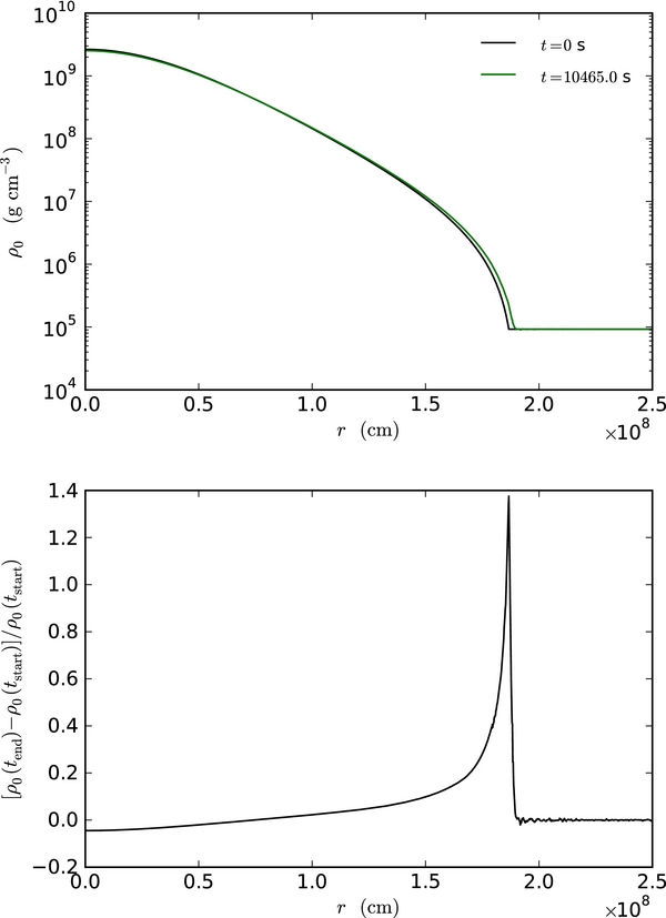
Figure 16. Top: base state density ρ0 as a function of radius at the start and end (ignition) of simulation A. Bottom: relative change in the base state density (start compared to ignition) for run A. We see that the density decreases slightly in the center of the star. The large relative change at the edge of the star reflects the fact that the star expanded slightly.
Download figure:
Standard image High-resolution image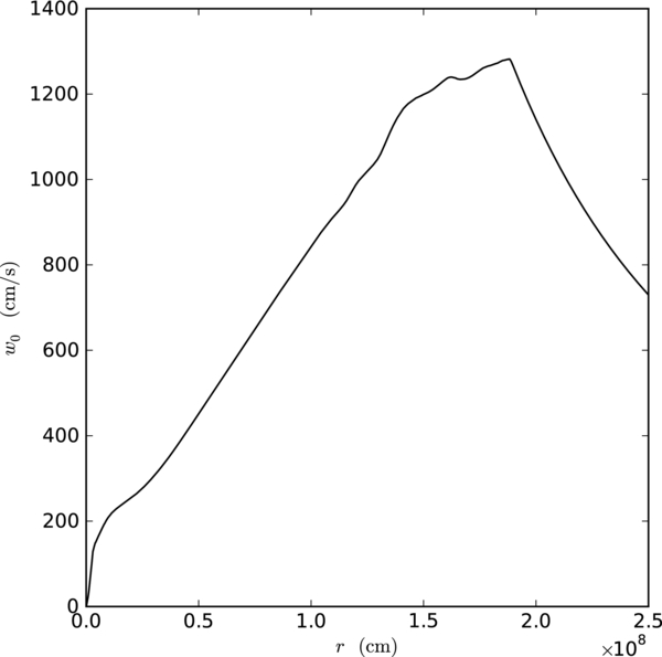
Figure 17. Base state expansion velocity, w0, as a function of radius at the end (∼1 s before ignition) of simulation A. Throughout the star, this velocity is many orders of magnitude smaller than the local velocity.
Download figure:
Standard image High-resolution image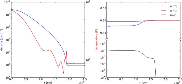
Figure 18. Average temperature and density (left) and composition (right) for simulation A ∼ 1 s before ignition.
Download figure:
Standard image High-resolution image3.2. Ignition Radius
Figures 19 and 20 show the hot spot radius as a function of time for calculations A through E for the 200 s preceding ignition. Since we define the radius as the distance from the cell center to the center of the star, the closest possible ignition radius, corresponding to the center of one of the eight zones with a vertex at the center of the star, is  (∼7.5 km for the 5763 simulation). Note that we are not tracking a particular parcel of fluid, but rather are recording the radius of the hottest cell at a given point in time (as a very hot parcel of fluid rises and cools, eventually a new, hotter parcel will form at a different location). In our figures, the time axis has been shifted by subtracting off the time at which ignition occurs, tignite. The red horizontal line is the average radial position for the interval t ∈ [tbegin, tend], where tbegin = −200 s and tend = −1 s, measured with respect to tignite. The choice of the end time for the average is to exclude the ignition itself, which will bias the results as the burning spreads artificially throughout the star. Our data consist of a collection of hot spot radii, Rn, and associated times, tn, where n refers to the time step. We perform a time-weighted average, where we take the position Rn to hold for the time interval
 ![$t\in [t^{n-{}^1/_2},t^{n+{}^1/_2}]$](https://content.cld.iop.org/journals/0004-637X/740/1/8/revision1/apj399128ieqn14.gif) , where tn ± 1/2 = (tn + tn ± 1)/2. Then the average hot spot radius,
, where tn ± 1/2 = (tn + tn ± 1)/2. Then the average hot spot radius,  , and its standard deviation, δRhot, are computed as

with
and nbegin is the time step corresponding to tbegin and nend is the time step corresponding to tend. In Table 2, we list these quantities for runs A through E, with tbegin = −200 and −100 s. These show that the average hot spot radius is about 50 km, with a standard deviation between 20 and 26 km. The main result from this table is that the statistics of the average hot spot location seem to agree for either starting time. It is not clear from these numbers if there is a trend that the rotating runs show a higher δR than the corresponding non-rotating case—this will need many more calculations to clearly understand.
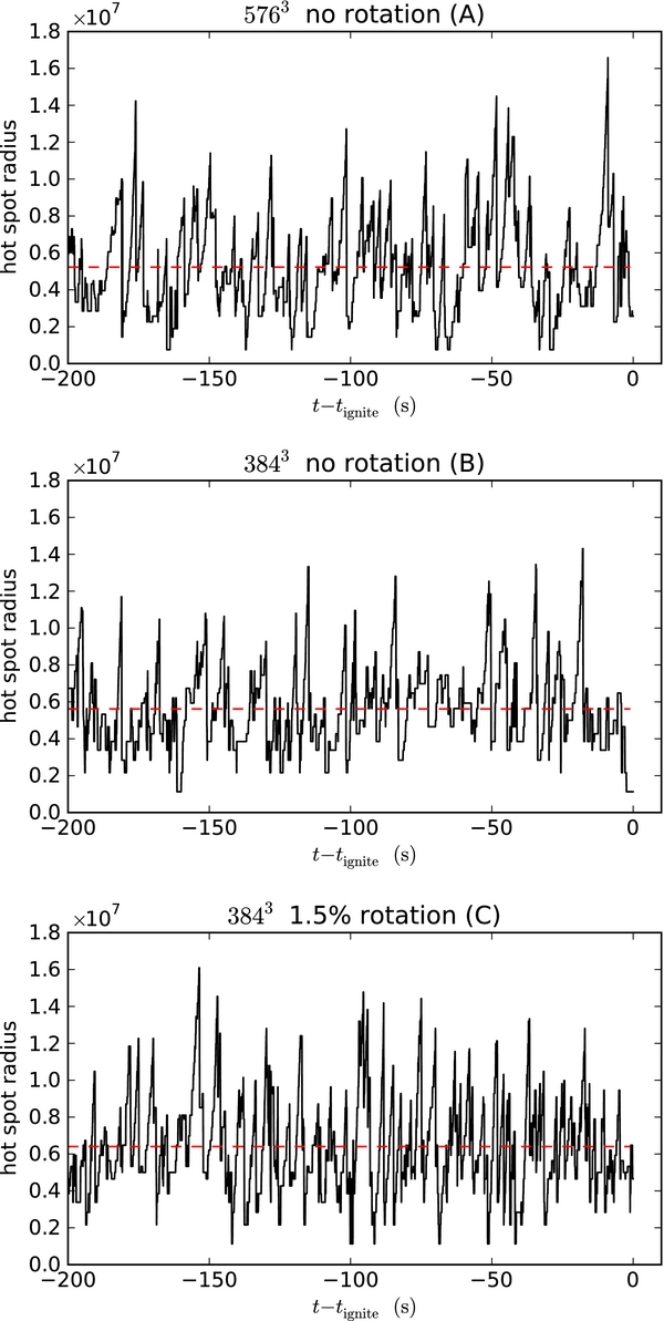
Figure 19. Radial location of the peak temperature as a function of time for runs A through C (top to bottom). Only the last 200 s before ignition are shown. Here, we see that right up to the end of the calculation the hot spot location changes rapidly. The horizontal red line indicates the average radial position of the hot spot from 200 s to 1 s before ignition.
Download figure:
Standard image High-resolution image
Figure 20. Radial location of the peak temperature as a function of time for both the non-rotating (top) and rotating (bottom) 2563 runs (D and E, respectively). Only the last 200 s before ignition are shown. The horizontal red line indicates the average radial position of the hot spot from 200 s to 1 s before ignition.
Download figure:
Standard image High-resolution imageTable 2. Time-averaged Hot Spot Location and Standard Deviation
| ID | tbegin = −200 | tbegin = −100 | ||||
|---|---|---|---|---|---|---|
 |
δR |  |
δR | |||
| (km) | (km) | (km) | (km) | |||
| A | 52.3 | 25.5 | 54.9 | 27.3 | ||
| B | 56.2 | 21.8 | 59.8 | 21.5 | ||
| C | 64.0 | 25.8 | 64.4 | 26.6 | ||
| D | 52.0 | 20.9 | 49.5 | 21.6 | ||
| E | 48.2 | 23.2 | 49.8 | 25.2 | ||
Download table as: ASCIITypeset image
We can try to get a clearer picture of the likely ignition radius by breaking the final approach to ignition into small time intervals and looking at a histogram of the properties. We pick a time interval, Δthist, over which to average the data, where Δthist is chosen to be larger than the characteristic time step used at this point in the simulation. As an example, for the 5763 simulation (A), Δthist = 1 s is a factor of ∼30 larger than a typical time step. Thus, data from many time steps will contribute to a single average used in the histograms. We then construct a piecewise-linear profile for the radius corresponding to the maximum temperature as a function of time from our simulation data, and compute the average radius over each time interval by integration. Figure 21 shows the resulting histogram for simulation A, considering only the last 200 s of data leading up to ignition (excluding the final 1 s). Several versions are shown, with all but one using Δthist = 1 s. The top left plot colors the intervals by the temperature of the hot spot averaged over the time interval. The general shape corresponds well to our expectations from Figure 19—the peak is around 50 km. Within each temperature interval, the overall shape of the distribution appears roughly the same, with a peak around 50 km and a slightly extended tail to higher radii, indicating that hot spots of all temperatures can appear at any radius in the distribution. The top right plot shows the same histograms, this time with the colors indicating the average radial velocity. We immediately see that the vast majority of hot spots are associated with outward moving flows. Only a handful of cases have vr < 0. Figure 21 also indicates a slight tendency for the hot spots at larger radii to be associated with larger values of vr—as expected, since the flow will carry them away from the center. To assess the robustness of these results, we can look at the dependence on the time to ignition and the size of Δthist. The bottom left histogram shows the same data but instead colored by time to ignition. Here, we see a reasonably symmetric distribution for all cases, indicating that the hot spot radius does not depend strongly on time to ignition. Finally, the bottom right histogram again shows the histogram colored according to vr (as in the top right), but using Δthist = 0.5 s instead of 1 s. The overall shape compares well to the Δthist = 1 s case, indicating that the results do not strongly depend on the length of the averaging interval.

Figure 21. Histogram of the likely ignition radius for the last 200 s preceding ignition for the 5763 simulation (A). All but the bottom right plot have Δthist = 1.0 s. Top left: the coloring shows the average T of the hot spot over the averaging interval. Top right: the coloring now shows the average vr over the averaging interval. Bottom left: the coloring shows the time to ignition of the averaging interval. Bottom right: again showing the average vr but now with Δthist = 0.5 s.
Download figure:
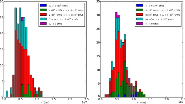
Standard image High-resolution imageFigure 22 shows the histograms for simulations B and C, colored according to vr. These histograms agree with the overall behavior seen in those for the main simulation (A).
Figure 22. Histogram of the likely ignition radius for the last 200 s preceding ignition, averaged over 1 s intervals, for the 3843 simulations B (left) and C (right). The coloring shows the average vr of the hot spot over the averaging interval.
Download figure:
Standard image High-resolution image
Overall, these histograms show that the hot spot is most likely to be found off-center, with a radius of ∼40–75 km most favored. There is an extended tail in the distribution toward higher radii. We also find that the vast majority of the hot spots have an outward moving velocity. We note a few caveats. First, at any instant, we only keep track of a single hot spot—wherever the temperature is greatest. For that spot, we record the position, velocity, and temperature. If a second spot somewhere else in the flow is only slightly cooler, we will not record it until it becomes hotter than the one we are following. Second, none of these spots ignited. They are all "failed" ignition points. If they were slightly hotter, they may have led to ignition, and therefore ended our calculation. Finally, there is a delay between when the hot spot forms and when it ignites (Garcia-Senz & Woosley 1995; Iapichino et al. 2006). We believe that we capture most of the evolution of the hot spot leading up to a potential ignition in these simulations, but any more evolution would correspond to a small displacement away from the center (since vr > 0). Overall, we believe that these histograms show us the distribution of "likely" ignition points. Taken together, we believe that these histograms closely reflect the distribution of ignition points, and suggest that off-center ignition is most likely.
As in Paper IV, we define ignition to be the time at which the peak temperature exceeds 8 × 10⁸ K, on its way to a steady rise to several billion Kelvin. Generally, once this temperature is reached, ignition is imminent. For run B, it takes only 0.71 s (17 time steps) for the temperature to go from 8 × 10⁸ K to 9 × 10⁸ K. Similarly, for run C, it takes 0.92 s (25 time steps) for this temperature increase. In both cases, the temperature reaches several billion Kelvin just a few steps later. At this point, physically, a flame should form; however, at the resolution of these studies we are very far from resolving the structure of that flame. Consequently, the reactions run away and predict a dramatic, non-physical increase in velocities and the numerics are no longer valid. In Table 1, we list the location of the first flame and the radial velocity in that zone, for each of the simulations presented to date. We note that all of the radial velocities are positive, indicating that at the time of ignition, the hot spot was moving away from the center. Unlike Höflich & Stein (2002), who find that ignition is "triggered by compressional heating near the white dwarf center," our results suggest that the ignition occurs when the hot spot is moving away from the center. We do not have any Lagrangian information on the fluid to tell what path it took to arrive at its present state, but it is likely that the hot spots arise when a fluid element is heated near the center and then buoyantly rises away, as discussed in Wunsch & Woosley (2004) and Woosley et al. (2004).
4. CONCLUSIONS AND DISCUSSION
The main results of this study are that the distribution of hot spots near the time of ignition suggests that off-center ignition is strongly favored, and that even a small amount of rotation appears to be enough to disrupt the dipole nature of the convective flow. Our results are qualitatively similar to those from Paper IV. The main difference is that in the present simulations, we do not see a breakdown of the transition between the convectively unstable and stable regions at late times. In the present simulations, up to the point of ignition, the convective region remains well defined. This new behavior keeps alive the possibility suggested by Piro & Chang (2008) that the transition of the burning front to a detonation may coincide with the flame crossing into the outer stable region.
The variety of outcomes from these simulations, taken together with those from Paper IV, reinforces the idea that ignition is a highly nonlinear behavior. Different simulations, with small differences in the initial conditions, lead to different ignition outcomes. Doing a large number of ignition calculations to build a statistical picture of the allowed radii of ignition points is prohibitively expensive. The 3843 calculations presented here required approximately 1 million CPU hours on the Cray XT5 machine at ORNL and the 5766 calculation required about 7 million hr on the same machine. Table 1 summarizes our knowledge thus far, listing the ignition characteristics of the simulations we presented here and those from Zingale et al. (2009). The histograms of likely ignition radius for the present calculations complement our previous findings. While some simulations are consistent with central ignition, the histograms indicate that off-center ignition is most likely.
The likely ignition radius distribution has interesting implications for the explosion itself. The peak of the likely ignition radius distribution is ∼50 km, which is beyond the radius where the flame might burn through the center before floating away (Zingale & Dursi 2007), especially considering the outward-flowing velocity of the hot spot. This result is slightly smaller than previous analytic and numerical estimates of the likely ignition radius, including Garcia-Senz & Woosley (1995) ("several hundred kilometers"), Woosley et al. (2004) ("150–200 km off-center"), and Wunsch & Woosley (2004) ("of order 100 km").
How the explosion actually proceeds, then, depends on the number of hot spots that ignite in close succession. Off-center ignition of a single flame can lead to a flame bubble breaking out of the side of the star, driving flows that interact on the antipodal point, and potentially igniting a surface detonation (Plewa et al. 2004; Röpke et al. 2007b). Observations have also recently found that some of the diversity of SNe Ia can be explained by slightly asymmetric explosions (Maeda et al. 2010), which may result from off-center ignition. We note that the current calculations say nothing about any subsequent, "second" ignition. If multiple ignitions occur in rapid succession, we would expect that the distribution found in this study would still apply. We cannot, however, infer the time delay for a subsequent ignition, since we only track a single hot spot at a time in the current simulations. The use of Lagrangian tracer particles may help track multiple hot spots in future simulations. Multiple off-center ignitions could leave a large fraction of the center unburned, perhaps setting the stage for a detonation (Bychkov & Liberman 1995).
It is also interesting to note that both the table of ignition radii and the histograms of likely ignition radius show that the ignition generally will occur in an outflow from the center (positive (vr)ignition), although we lack any Lagrangian history to understand precisely how it reached this location. Again, we plan to use tracer particles in future simulations to provide that understanding.
A final finding from this work is that we need to continue to explore resolution. Turbulence should dominate the convection, as the Reynolds number in the star is O(1014) (Woosley et al. 2004). Estimating the numerical Reynolds number we attain is difficult, since we are not explicitly modeling viscosity. These current calculations do not yet show a well-resolved turbulent cascade. In future calculations, we will continue to push the resolution higher to understand the sensitivity of the ignition process to Reynolds number and the turbulent velocity field. We have already begun a follow-up calculation that will begin with the 5763 base grid, and add resolution near ignition using adaptive mesh refinement (AMR) to bring us to 1–2 km resolution at ignition. We will also perform a rotating counterpart at these resolutions. This calculation will be the focus of a forthcoming paper, where we examine the turbulent properties of the convective field.
Other future directions for ignition studies include examining the role of the 12C + 12C rate and initial model on the ignition outcome. Recent work by Cooper et al. (2009) proposes the existence of a resonance in this rate, motivated by observations of superbursts in accreting neutron star systems. They suggest there that the effect may be small. Iapichino & Lesaffre (2010) study the role of this rate on SNe Ia ignition and find that it can affect the ignition density. Using our framework, we can perform more detailed studies of the ignition process using different initial models and rates to see how large of an effect this rate has on the ultimate ignition. Binary evolution can yield Chandrasekhar mass white dwarfs with a large spread in central densities (Lesaffre et al. 2006), which can in turn affect the reaction rates and perhaps the distribution of ignition points.
The next major step beyond simply modeling the convection and first ignition is to evolve the system past the ignition of the first flame. There are several approaches that we can explore. Currently, when the first flame ignites, we do not have the resolution to accurately represent the flame propagation, which leads to enormous (and unphysical) velocities, and the simulation is no longer valid. One simple path to prevent this occurrence is to try turning off the burning once the temperature rises beyond a threshold (like 109 K). This is unphysical, but it may allow for the simulation to proceed for a short time without the first ignition point polluting the rest of the flow. If so, this can give a sense of where, and how far behind in time, the second ignition is. A more elegant solution is to restart this calculation in a compressible code just before the ignition. The CASTRO code (Almgren et al. 2010b) uses the same AMR library and microphysics, and allows for a such restart capability. We have begun to explore this restart capability for simple two-dimensional test problems (Almgren et al. 2010a). A final, longer term solution would be to incorporate a turbulent flame model into the low Mach number model that could accurately capture the evolution of the flame. In this context, the low Mach number model may need to be extended to include long wavelength acoustics to represent large-scale deformations of the star during the deflagration. Models of this type have been developed for atmospheric flows (Durran 2008), but they would need to reformulated for our system of equations.
We thank Alan Calder for many useful conversations about these simulations and their presentation here. We thank Jonathan Dursi for many helpful comments on an early draft of this paper. We thank David Chamulak and Ed Brown for helpful discussions regarding the energetics of the reaction network, and Frank Timmes for making his equation of state routines publicly available and for helpful discussions on the thermodynamics. We thank Andy Aspden for helpful input on diagnostics for these calculations. Finally we thank the anonymous referee for many useful comments on the paper. The work at Stony Brook was supported by a DOE/Office of Nuclear Physics grant No. DE-FG02-06ER41448 to Stony Brook. The work at LBNL was supported by the SciDAC Program of the DOE Office of High Energy Physics and by the Applied Mathematics Program of the DOE Office of Advance Scientific Computing Research under U.S. Department of Energy under contract No. DE-AC02-05CH11231. The work at UCSC was supported by the DOE SciDAC program, under grant No. DE-FC02-06ER41438 and the NASA Theory Program (NNX09AK36G).
Computer time for the main calculations in this paper was provided through a DOE INCITE award at the Oak Ridge Leadership Computational Facility (OLCF) at Oak Ridge National Laboratory, which is supported by the Office of Science of the U.S. Department of Energy under Contract No. DE-AC05-00OR22725. Computer time for the supporting calculations presented here was provided by Livermore Computing's Atlas machine through LLNL's Multiprogrammatic & Institutional Computing Program. Some visualizations were performed using the VisIt package. We thank Gunther Weber and Hank Childs for their assistance with VisIt.