


ABSTRACT
Some of the most challenging observations to explain in the context of existing flare models are those related to the lower atmosphere and below the solar surface. Such observations, including changes in the photospheric magnetic field and seismic emission, indicate the poorly understood connections between energy release in the corona and its impact in the photosphere and the solar interior. Using data from Hinode, TRACE, RHESSI, and GONG we study the temporal and spatial evolution of the 2006 December 14 X-class flare in the chromosphere, photosphere, and the solar interior. We investigate the connections between the emission at various atmospheric depths, including acoustic signatures obtained by time–distance and holography methods from the GONG data. We report the horizontal displacements observed in the photosphere linked to the timing and locations of the acoustic signatures we believe to be associated with this flare, their vertical and horizontal displacement velocities, and their potential implications for current models of flare dynamics.
Export citation and abstract BibTeX RIS
1. INTRODUCTION
During the last decade it has become well established that flares can and do impact the solar interior, as first predicted by Wolff (1972). The first observations of a "sunquake" were reported by Kosovichev & Zharkova (1998) during the flare of 1996 July 9, which strongly reinforced the foundations of local helioseismology and provided an additional stimulus for developing its methods further. Since that first identification by time–distance (TD) methods, the development of helioseismic holography has led to the identification of many more seismic sources during flares of GOES-class M and X (e.g., Donea et al. 2006; Zharkova & Zharkov 2007; Martínez-Oliveros et al. 2008b). Solar quake observations provide us with unique opportunities to study the excitation of solar oscillations in detail, and raise new questions about the underlying physical processes as well as the properties of the excited waves and sources producing them.
Similarly, confirmation that the photospheric magnetic field routinely changes during flares, both on short timescales (i.e., the duration of the impulsive phase) and longer timescales of hours (before and after a flare) has also become evident in the last decade through the studies by Kosovichev & Zharkova (2001), Zharkova et al. (2005), and Sudol & Harvey (2005, and references therein). Both solar quakes and transient magnetic changes occur during the flare impulsive phase, and, thus, appear in many occasions closely related to the initial energy release, and the appearance of enhanced continuum (WL) and hard X-ray (HXR) emission. More long-term magnetic changes (timescales of hours) similarly appear to begin during the impulsive phase and to have a good spatial relationship with WL and HXR emission. This has led to much discussion of the origins of quakes and magnetic changes in the context of electron precipitation in the thick target model.
The primary explanations for the origin of acoustic emission during flares have been well summarized by Lindsey & Donea (2008) and Zharkova (2008) and include: chromospheric shocks which arise as the result of the pressure transients driven by the hydrodynamic response of the ambient plasma to the precipitation of energetic particles (electrons or protons) into the chromosphere (e.g., Kosovichev & Zharkova 1995, 1998; Kosovichev 2006; Zharkova & Zharkov 2007; Donea & Lindsey 2005), pressure transients that are related to backwarming of the photosphere by enhanced chromospheric radiation (e.g., Lindsey & Braun 2000; Donea et al. 1999; Donea & Lindsey 2005), the Lorentz force transients that occur as a result of the coronal restructuring of the magnetic field (e.g. Hudson et al. 2008), and the precipitation of electron beams (Zharkova & Kosovichev 2002). These beams themselves carry a strong electric field (Zharkova & Gordovskyy 2006) that in turn can induce an electromagnetic field in the ambient plasma (van den Oord 1990) which modifies the magnetic field of the loop where particles precipitate.
The shocks formed by a hydrodynamic response of the ambient plasma to the precipitation of electron or proton beams seem to be good candidates for the formation of seismic ridges associated with solar flares since they carry sufficient momentum and energy that can be deposited in the solar photosphere (Kosovichev & Zharkova 1998; Zharkova & Zharkov 2007), but the question still remains open as to how exactly these shocks deposit their energy into the solar interior (e.g., depths, timescale) and how they can be accounted for from a detailed comparison with seismic observations. These are closely related to the other implications of particle precipitation into a flaring loop, like the formation of magnetic transients (Hudson et al. 2008) and non-thermal plasma ionization (Zharkova 2008).
In the case of magnetic changes Lindsey & Donea (2008) highlight that it is the transient component of magnetic changes that is the most relevant to acoustic emission, i.e., those changes that occur on a timescale of τ ≈ 2H/c or less, where H is the density scale height and c is the sound speed. In the photosphere this timescale is of the order of 40 s. The question of whether these short-term transient changes during the impulsive phase can be considered to represent a genuine change in the photospheric magnetic field is still a matter for debate, and the localized sign reversals, or "magnetic anomalies" (e.g., Qiu et al. 2002) are most often attributed to changes in the line profile occurring as the result of the sudden heating of the ambient plasma or by direct bombardment by high energy particles. In the case of the Ni 6768 Å line used by both GONG and the Michelson Doppler Imager (MDI) to make magnetic measurements, non-LTE simulations have shown that sudden heating is insufficient to turn this line into emission and that a large increase in electron density is required, i.e., intense particle bombardment (Zharkova & Kosovichev 2002). Observations by Qiu & Gary (2003) that find a good correspondence between the HXR sources and magnetic anomalies lend support to the hypothesis that magnetic field changes are associated with energetic particles. However, simulations of GONG and MDI observations by Edelman et al. (2004) also conclude that magnetic measurements are less sensitive to the changes in the line profile than Doppler measurements. Nevertheless, we caution that it is likely that the radiative environment during the impulsive phase of a flare will affect both Doppler and magnetic signatures, and this should be kept in mind when interpreting changes in these parameters.
Recently, Martínez-Oliveros & Donea (2009) examined the relationship between magnetic field changes and seismic emission in two acoustically active flares and found there was no clear connection between the acoustic emission observed in the 5–7 mHz range and magnetic transients in one of the events, while in the other flare the acoustic sources were found in the vicinity of the magnetic transients. They also noted that there are many flares that show magnetic changes but no detectable acoustic emission (Martínez-Oliveros & Donea 2009). Thus, while it appears there are many common connections and overlaps in the phenomena described above, there are equally many unresolved questions regarding causal connections.
In this paper we present high-resolution observations of the X-class flare of 2006 December 14. Our data set is comprised of observations of the chromosphere and photosphere (including the magnetic field) from Hinode and TRACE, intensity and velocity data from GONG, and HXR observations from RHESSI. We present tentative evidence for flare-related acoustic signatures in the GONG data which, although weaker than those seen with MDI, indicate the probable existence of a sunquake. In Section 2 we first outline the flare morphology and evolution at multiple wavelengths, discussing in Section 2.2 the relationship between the various signatures seen in the photosphere and the chromosphere. In Section 3 we discuss the TD and acoustic holography methods that we believe indicate that the flare is acoustically active, and the caveats associated with them. We also investigate the flare-related velocity signatures measured by Hinode in the photosphere and their possible role in the flare dynamics.
2. OBSERVATIONS
2.1. Description of the Data
The flare on 2006 December 14 originated from active region (AR) 10930 and occurred at approximately 22:00 UT. The X-ray flux for the event peaked at GOES X1.5 level around 22:12 UT. The event was observed by all the instruments on the Hinode spacecraft (Kosugi et al. 2007). In this paper we focus primarily on the observations made by the Solar Optical Telescope (SOT; Tsuneta et al. 2008). The SOT observed the flare throughout its duration with the Broad-band Filter Imager (BFI) in the G band and Ca ii H line, with a 2 minute cadence and 0.1 arcsec resolution. It also observed with the Narrow-band Filter Imager (NFI). The NFI consists of a tunable Lyot filter preceded by wide-band interference filters that cover six spectral regions. The bandpass of the Lyot filter is sufficiently narrow (95 mÅ at 630 nm) to allow magnetogram and Dopplergram measurements to be made in the available spectral lines, and by operating in synchronous mode with the polarization modulator of SOT, the NFI is able to make Stokes I, Q, U, and V images. In this work we use the Stokes I and V images integrated over the Fe i 6302 Å passband with an approximately two-minute cadence and 0.16 arcsec resolution. These represent the intensity (I) of the beam in this wavelength range and, as noted in Landi Degl'Innocenti & Landi Degl'Innocenti (1973), the circular polarization, V, is particularly suitable for measuring the longitudinal component of the magnetic field. The SOT polarization model (Ichimoto et al. 2008) indicates that the NFI observed parameters I' and V' are related to the Stokes parameters I and V by the following relations: I ≈ I' + 0.481Q and V ≈ V'/(− 0.798). Since Q is not measured we have to neglect cross talk between Q and I and let I ≈ I'. Chae et al. (2007) estimate that this will introduce an approximately 10% error in sunspot penumbrae. However, since our main purpose for these data in the current work is to determine polarity and temporal changes rather than magnitude of the longitudinal field, as well as the location and timing of emission enhancements in the Fe i passband, for which the NFI provides much higher cadence, we are satisfied that this does not compromise our results. For simplicity we will henceforth refer to measurements of V from the NFI as the longitudinal magnetic field, with the caveat that these represent polarity but not magnitude of the field. Standard corrections were made to these data for CCD gain, readout defects, dark current, and pedestal. The data were aligned using cross-correlation and sub-pixel registration on a large field of view (FOV) similarly to the method described in Gosain et al. (2009). The alignment was verified through visual inspection of running difference images which showed random orientation of dipolar features within the FOV.
The spectro-polarimeter (SP) is a modified Littrow spectrometer that records two spectra in orthogonal polarization states simultaneously. The raw spectra are then added or subtracted onboard in order to de-modulate the Stokes I, Q, U, and V spectra in each of the orthogonal polarization states. The SP performed fast map scans of the active region with 0 32 resolution and a duration of 32 minutes. The time per slit position was 3.2 s. The data were corrected for dark current, flat field, and cosmic rays using standard SolarSoft routines, and the Stokes profiles obtained in the Fe i 6301.5 and 6302.5 Å lines were inverted using the full atmosphere inversion code LILIA (Socas-Navarro 2001). The inversion provides inferred values of atmospheric parameters such as velocity and the magnetic field vector through least-squares fitting of the observed Stokes profiles. Its primary assumptions are a one-dimensional plane–parallel atmosphere, LTE, and hydrostatic equilibrium. The intrinsic 180° ambiguity was resolved using the Automated Ambiguity resolution code (AMBIG; Leka et al. 2009) which is based on the Minimum Energy Algorithm (Metcalf 1994).
RHESSI observed the flare from its beginning until approximately 22:25 UT and we used the CLEAN algorithm to produce images at one-minute time intervals from 22:08 to 22:15 UT, using the same procedure described by Watanabe et al. (2010).
GONG observations during the period were made in the photospheric Ni i 6768 Å line with one-minute cadence. The observations included full-disk Dopplergrams, line-of-sight magnetograms, and intensity images. The pixel size of the intensity images is 2.5 arcsec. In this study we use line-of-sight Dopplergrams to analyze the acoustic signatures of the flare through both the time–distance diagram technique (TD method; Kosovichev & Zharkova 1998) and acoustic holography (e.g., Lindsey & Braun 2000). We have also used intensity images to compensate velocity measurements for atmospheric distortion by applying the cleaning procedures outlined in Lindsey & Donea (2008).
2.2. Flare Morphology and Evolution
The flare exhibited extended ribbon emission that propagated through the umbrae and penumbrae of both the northern and southern spots. This emission was seen in multiple wavelengths, as shown in Figure 1, where we plot a series of running difference images that display the temporal and spatial evolution of the flare in the G band, the intensity measured in the Fe i 6302 Å passband (I measured by the NFI), the circular polarization V (which is proportional to the longitudinal magnetic field), the Ca ii H line, and the TRACE WL channel. As can be seen from this figure the morphology and location of the emission seen in the G band and the I and V components measured in the Fe i 6302 Å passband are almost identical. The emission in the G band is somewhat stronger than in the I and V components, and clear reversals of the field are seen in the longitudinal magnetic field. TRACE's WL channel has a broad response which includes a contribution from the UV (Fletcher et al. 2007), and as a result the emission in this band is more extended than the photospheric G band and Fe i 6302 Å emissions. The Ca ii H line difference images show that the photospheric emission forms a more compact subset of the chromospheric emission, but that it is spatially coincident. These observations clearly indicate that energy deposition at the photospheric level occurs over a more confined area than the overlying chromosphere.

Figure 1. Running differences in descending order of the images taken in: integrated intensity Fe i 6302 Å passband (Stokes I); longitudinal magnetic field (Stokes V); G band; Ca ii H; TRACE WL intensity. See the text for details of I and V.
Download figure:
Standard image High-resolution imageIn Figure 2 we illustrate the temporal evolution of the flare in the 40–100 keV HXR energy range (solid line, spatially integrated flux) and in the G band in the southern (diamonds) and northern (asterisks) flare ribbons. The intensity has been normalized by area and scaled for easier comparison, but the strongest emission in the G band is seen in the southern ribbon, as also noted by Watanabe et al. (2010). In Figure 3 we display images of the HXR emission reconstructed using the CLEAN algorithm in the 20–30 keV energy range. Overlaid on these images are the contours of the 20–30 keV emission at the 50% and 70% levels (cyan) and the 40–100 keV emission at the same levels (orange). This demonstrates that as well as an asymmetry in intensity of the HXR sources, there is an asymmetry in size. In particular, one can note that the northern 20–30 keV HXR source recorded at 22:08 UT was smaller than the southern one. However, at 22:09 UT the southern HXR source had grown to a similar size to the northern one and is larger for all the subsequent times up to 22:15 UT.

Figure 2. Temporal evolution of the 40–100 keV HXR emission (solid line) and G-band emission in the two southern sources (diamonds) and in the two northern sources (asterisks). The intensity was scaled to aid a visual comparison of the curves.
Download figure:
Standard image High-resolution image
Figure 3. Time series of HXR images from 22:08 to 22:15 UT on 2006 December 14. The gray-scale images are 20–30 keV, with overlying contours (cyan) showing the emission at 50% and 70% of the peak. The orange contours show the 40–100 keV emission at the same levels.
Download figure:
Standard image High-resolution imageFigure 4 shows on the left an image of the pre-flare magnetic field. The image in the center shows the changes in the longitudinal magnetic field derived from running difference (22:11 and 22:09 UT in this case) as blue contours on a magnetogram taken at 22:09 UT. The location of the HXR emission in the 50–100 keV energy range is overplotted with orange contours. The right panel of this figure shows regions of interest that were selected around the magnetic reversals and the outer edges of the G-band ribbons, regions 1–4. Region 5 was chosen as a reference point away from the main flare disturbance. The temporal evolution of the longitudinal magnetic field in regions 1–4 can be seen in Figure 5. We see strong impulsive changes in magnetic flux at the time of the flare in the regions 1 and 4, and a step change in regions 2 and 3.
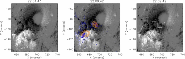
Figure 4. NFI images of the pre-flare longitudinal magnetic field (left plot); the longitudinal field measured during the flare overplotted with the contours of 50–100 keV HXR emission seen by RHESSI (orange) and blue contours of the magnetic field difference (22:11–22:09 UT) (center plot); magnetogram indicating the regions of interest (1–4) associated with the flare-related magnetic changes and the G-band ribbons. Region 5 represents a reference region away from the main flare disturbance (at the very bottom of the right plot).
Download figure:
Standard image High-resolution image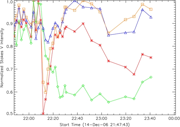
Figure 5. Normalized Stokes V intensity (longitudinal magnetic field) in regions 1 (red asterisks), 2 (green diamonds), 3 (blue triangles), and 4 (orange squares) as indicated in Figure 4.
Download figure:
Standard image High-resolution image2.3. Underlying Magnetic Field Configuration
SOT's SP performed fast map scans of the active region before, during, and after the flare. The SP scans from east to west, and the scans began at 17:00 and 22:00 UT on the December 14 and 05:45 UT on the December 15, taking 32 minutes to complete. The FOV covered 1000 slit positions with a spatial resolution of 0.32 arcsec. In Figure 6 we show the absolute magnetic field strength (derived from the inversion) in the active region at 17:00 (top left), 22:00 (top center), and 05:45 UT (top right), and the magnetic field inclination with respect to the line of sight at the same times (also derived from the inversion). An inclination of 90° indicates a field perpendicular to the local vertical. The four boxes correspond to the regions 1–4 shown in Figure 4.
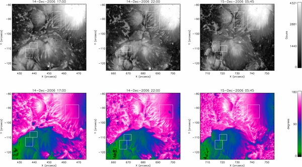
Figure 6. Top: absolute magnetic field strength in Gauss at 17:00 (left) and 22:00 UT (center) on the 2006 December 14, and 05:45 UT (left) on the December 15. Bottom: magnetic field inclination at corresponding times. The boxes are the locations of regions 1–4 shown in Figure 4.
Download figure:
Standard image High-resolution imageIt can be seen that there are significant variations during the period of the three scans, which is some 12 hr in total. The large length of time between the scans of the region makes it difficult to say with certainty, which changes occur as a direct result of the flare, and which are due to a "normal" evolution of the active region. However, the map of inclined magnetic field taken during the course of the flare shows new localized regions of 90° inclination in all four regions, but particularly in regions 2 and 4. These have diminished or disappeared in the scan taken on December 15 at 05:45 UT. In terms of magnetic field strength, all the regions show a mix of field strengths, with the majority ranging between 1000 and 2000 G. Region 4 in the north includes the highest field strength, approaching 4000 G. There appears to be significant weakening of the field in all regions in the scan taken at 05:45 on December 15, consistent with the overall trends seen in Figure 5.
3. HELIOSEISMIC OBSERVATIONS
3.1. Description of Basic Techniques
In order to detect and analyze a possible solar quake associated with the flare we use both TD analysis (Kosovichev & Zharkova 1998) and acoustic holography (Donea et al. 1999). TD analysis is applied to detect the circular ripples generated on the solar surface by a quake. This consists of rewriting the observed surface signal in polar coordinates relative to the source, i.e., v(r, θ, t), and using azimuthal transformation
where m defines the wave type. In the current paper we investigate only a circular wave component, e.g., using the case when m = 0, and look for evidence of the propagating circular wave. Then if seen, the quake manifests itself as a TD ridge, thus providing estimates of the surface propagation speed and the time of excitation. In this work the GONG high-cadence velocity data were used in the TD analysis.
Acoustic holography is applied to calculate the egression power maps from observations. The holography method (Braun & Lindsey 1999, 2000; Donea et al. 1999; Lindsey & Braun 2000) works by essentially "backtracking" the observed surface signal, ψ(r, t), by using Green's function, G+(|r − r'|, t − t'), which prescribes the acoustic wave propagation from a point source. This allows us to reconstruct egression images showing the subsurface acoustic sources and sinks:
where a, b define the holographic pupil. The egression power is then defined as
In this work, Green's functions built using a geometrical optics approach were used, pupil dimensions were defined a ≈ 15 Mm, b ≈ 55 Mm, with GONG Dopplergram velocity data taken as ψ(r, t) for the egression power calculations.
3.2. 2006 December 14 Helioseismic Results
Since there are no suitable SOHO/MDI observations available during the flare period we have obtained intensity and Dopplergram data from the GONG network (Harvey et al. 1996). The comparison of results of the TD method and acoustic holography when applied to SOHO MDI and GONG velocity data has been carried out in Zharkov et al. (2011) by looking at three acoustically active flares for which the data from both instruments were available. It has been established that while the GONG data are much noisier, after the GONG-specific correction procedures, traces of acoustically active flares can be detected in the computed egression power snapshots and TD diagrams.
Two GONG data sets are used in our analysis consisting of several hours of full-disk one-minute cadence intensity and line-of-sight velocity observations starting at 22:00 UT, 2006 December 14. Each series was processed by tracking and de-rotating the region of interest centered on the active region using the Snodgrass rotation rate, and then remapping the data onto heliographic grid at 0 15 pixel−1 resolution. To compensate for the atmospheric contribution we use the cleaning procedures described in Lindsey & Donea (2008) for GONG intensity data. Since both the intensity and velocity data come from the same instrument, we apply the parameters extracted from the intensity series to correct the line-of-sight velocity data. In addition, we apply an acoustic power map correction to the GONG velocity data following the procedure described by Zharkov et al. (2011) for the egression power measurements.
The egression power snapshots computed from the corrected Dopplergram series are plotted in Figure 7. The left column shows the egression maps for 22:07 UT and 22:12 UT with arrows indicating the location of the ripples measured from the TD diagram (Figure 8). The right column shows close-ups of the egression power for the same times. The white contours indicate the outline of the sunspot and the black contours represent 2.02, 2.25, and 3 times the mean quiet Sun egression power. The close-ups show possible traces of acoustic activity at the four locations coinciding with the locations of fast magnetic field changes reported in Figures 4 and 5; the links are explicitly shown in Figure 9.

Figure 7. Left: egression power snapshots (4–6 mHz) taken around 22:07 UT (upper row) and 22:12 UT (bottom row) derived from GONG Doppler data. Carrington longitude is along the x-axis, latitude is along y-axis. The TD source location is indicated by the arrow. Right: close-ups of the flare region at the same times: white contours are those of the sunspot penumbra and black contours are 2.02, 2.35, and 3 times the mean quiet Sun egression power.
Download figure:
Standard image High-resolution image
Figure 8. Time–distance diagram for the 2006 December 14 flare northern source (left) with theoretical travel time ridge corresponding to l = 1000 overplotted using the white dashed line (right).
Download figure:
Standard image High-resolution image
Figure 9. Left: gray-scale difference image of the flare in the G band, with contours of the sunspot overlaid in white. Contours of the 20–30 keV HXR emission are shown in red, and 40–100 keV in yellow. The thick black contours show 2.02, 2.35, and 3 times the mean quiet Sun egression power. The numbers are related to the similarly numbered boxes defined in Figure 4. Right: the same contours overplotted on a Ca ii image showing the cooling flare arcade. Note that we have masked the sunspot (shown by the white contour) to suppress the quiet Sun egression power, in order to make the flare-related emission easier to identify.
Download figure:
Standard image High-resolution imageIn order to detect ripples associated with acoustic waves occurring beneath regions 1–4 for the 2006 December 14 flare, at first we searched for ridges in the TD plots in the locations of all regions showing magnetic changes. TD diagrams were computed from the GONG Dopplergrams at the locations 10 × 10 pixels around each region in the south and north. From 100 TD diagrams we searched for ridges corresponding to the propagation of a circular wave produced by a spherical seismic wave in the solar interior excited by the flare. We found that a detectable TD ridge corresponding to a circular wave was located only in the location of the largest egression power source in region 3 around 84 Carrington longitude and 525 latitude south (see Figure 8, left). The ridge is fitted reasonably well by the theoretical ridge (Figure 8, right) corresponding to the spherical wave number l = 1000 (which is the same as observed in the very first sunquake Kosovichev & Zharkova 1998), with the quake start time estimated at around 22:10 UT. There are some remnants of a ridge seen in TD diagram for the egression source in region 4 which we do not plot here. We are not able to reliably identify with the TD method any visible acoustic sources at the southern egression source locations 1 and 2, perhaps due to different physical conditions in these locations and the strong transient magnetic field variations and atmospheric contribution present in the GONG velocity observations (Lindsey & Donea 2008; Zharkov et al. 2011).
In Figure 9 we overplot the contours of the HXR emission (red: 20–30 keV, yellow: 40–100 keV) and the egression power (black: 2.02, 2.35, and 3 times mean quiet Sun) on a G-band difference image depicting WL emission (left plot) and on a Ca ii image from 22:44 UT (right plot). In order to avoid a confusion with the quiet Sun acoustic emission, the sunspot is masked out so that only the flare-related egression power is shown.
Figure 9 shows that the egression signatures in regions 1–4 are closely correlated spatially with the ends (or footpoints) of the two flaring loops seen in Ca ii emission. It can be also noted that the traces of egression power seen in the magnetic transient regions 1 and 2 coincide well with the southern HXR emission locations for the energies above 40 keV, while the smaller northern egression source detected in the location of magnetic transient 4 coincides with the end of the WL ribbon and HXR emission in the range 40–100 keV. Keeping in mind that the egression sources 1, 2, and 4 are weak, and since the GONG data are noisy, we will at best speculate on the reality of these sources.
Most interesting case is with the largest acoustic kernel 3 seen in the north, which coincides with the step-like change in magnetic field in region 3, and with the location of the center of the TD source (see Figure 8). However, the source 3 does not show close correspondence to any HXR sources. This appears to be one of the very rare cases resembling the one reported recently for the flare of 2011 February 15 (Kosovichev 2011). For the validation of the egression source 3 we can check its statistical significance as discussed below.
3.2.1. Statistical Significance of Seismic Signatures
We appreciate that acoustic signals detected from GONG data are generally noisier than the results obtained from space-based SOHO/MDI instrument as established earlier by Zharkov et al. (2011). On the other hand, the acoustic holography technique appears to be more sensitive to noisy signals present in Dopplergrams compared to the TD one, even when using the better quality SOHO/MDI data, thus detecting a greater number of quakes (see for instance Donea & Lindsey 2005; Besliu-Ionescu et al. 2005; Lindsey & Donea 2008). For the flare of 2006 December 14 we note that the egression signatures derived from the GONG data are close to those detected by MDI for M-class flares (compare the egression power plots for the M9.5 class flare in Figure 5 of Donea et al. (2006) or in Figures 2 and 3 of Martínez-Oliveros et al. (2008a) for M6.5 class flare with those presented here in Figure 7 for this X1.1 flare measured by GONG).
The fact that we see acoustic signatures at the same location in the north derived from both the TD diagram and egression power snapshot methods leads us to believe that such signatures can be real and not generated by background noise, as we demonstrate in the Appendix. In order to test this argument, we, similarly to Donea et al. (2006; their Figure 5), plot the egression powers at 3 and 6 mHz versus time integrated over the rectangular region indicated in Figure 10 centered on acoustic source 3. It can be seen in Figure 10 that the peak of the egression power at 6 mHz corresponds to the time of the strongest HXR source in the north, which is observed around 22:10 UT, i.e., slightly later than the start of integrated HXR emission (see Figure 2). This is in spite of a limited bandpass of the egression acoustic power computations (e.g., the egression power signatures is temporally smeared by ≈500 s) imposed by the filtering in 5–7 mHz frequency band used in the processing for GONG data (Donea & Lindsey 2005). Furthermore, the peaks approach the magnitudes of 2.5 and 3.85 for the frequencies 3 and 6 mHz, respectively, very close to the peak magnitudes (2.5 and 4) reported by Donea et al. (2006) for the flare of 2001 September 9, or those of 2.3 and 2.7 reported for the same frequencies by Martínez-Oliveros et al. (2008a).
Again following the analysis of Donea et al. (2006) and Martínez-Oliveros et al. (2008a), we also estimate the rms deviations, σ, from the mean in the strongest seismic source detected in the location of the flare and compare them with those detected in quiet Sun locations. In the Appendix we produce a statistical analysis of the quiet Sun region located on the same latitude but at plus 180° of the flare longitude. We do find some peaks of comparable magnitude to our source in the quiet Sun, but we estimate that the probability of a seismic source of magnitude of 3.85 being produced by sporadic noise is about 0.047% (see Figure 13 and its discussion in the Appendix). Therefore, it is likely that, at least, some of the peaks present in the quiet Sun egression computation might correspond to real seismic sources caused by turbulent convection (Deubner et al. 1992; Gizon et al. 2010).
On the other hand, the seismic (egression) sources associated with the flare cannot be attributed to convective turbulence, since they are located inside sunspot penumbrae which are characterized by strong magnetic field inhibiting such convection. Furthermore, these possible seismic sources are also spatially associated with the regions displaying fast magnetic field variations at the onset and for the duration of the flare, three of which (regions 1, 2, and 4) overlap in space with the HXR emission locations. Therefore, this gives us a reason to believe that the acoustic emission associated with these four locations in the flare may correspond to sunquakes excited by the processes occurred during the course of the flare. All four of the seismic sources are also co-spatial with WL emission, although we note that the strongest acoustic source 3 does not correspond well with the strongest WL emission similar to the situation reported recently for the flare of 2011 February 15 (Kosovichev 2011) that has yet to be interpreted in the context of existing models.
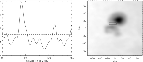
Figure 10. Left plot: 6 mHz egression power for the source in region 3 vs. time, integrated over the rectangular region in the intensity. Right plot: the Postel-remapped GONG intensity with the box indicating the area over which the integration was made.
Download figure:
Standard image High-resolution imageIn addition, we see a TD ridge at the location of the egression source in region 3 of the flare. Again, because the TD location is inside a strong magnetic region, the acoustic emission there cannot be attributed to stochastic convective turbulence which is suppressed by this magnetic field. Thus, it is either a true sunquake signature or is due to spurious noise. Repeating our integration procedure for the control quiet Sun data cube (see the Appendix) shows that the probability of a sporadic occurrence of this seismic source is very small (<4.7 × 10⁻⁴); thus, it has to be the one associated with the flare. Unsurprisingly, we have not been able to detect any TD ridges at the locations of the quiet Sun egression peaks. The fact that the egression signatures are relatively weak can probably be best explained by the fact that the strength of acoustic sources derived from the holographic technique with the filter centered at 5–7 mHz can suppress any acoustic oscillations at lower frequencies (3–5 mHz) which contribute substantially to the detection of the ridge in the source 3 with TD diagram technique. Recall that for this flare we see the TD ridge in the unfiltered data that obviously includes lower frequency oscillations.
As far as we are aware, so far for every quake detected with TD ridges there was associated acoustic emission detected via egression analysis (1996 July 9, Kosovichev & Zharkova 1998; 2001 March 10, Martínez-Oliveros & Donea 2009; 2003 October 28, Zharkova & Zharkov 2007; Donea et al. 1999; 2005 January 15, Martínez-Oliveros et al. 2008b; Moradi et al. 2007). Moreover, it can be argued that this might generally be the case, since the egression computation uses virtually the same data and should revert the anomalous wave-field fluctuations seen as a TD ridge to a source. Obviously, the reverse is not true, since the holography technique is naturally more sensitive in picking up acoustic signatures from wave-field observations. This could explain the lack of ridges seen in the egression signatures seen in regions 1, 2 and the weak half-ridge seen associated with the signature in region 4.
3.3. Motion in the Photosphere
Hinode's SOT also allows us to investigate how the photospheric velocity field changes during the course of the flare. The active region, as noted above, was observed at approximately two-minute cadence by both the NFI and the BFI. The SP also performed a scan of the region, as we describe above, but unfortunately did not cover the flare region until 22:35 UT, well after the impulsive phase and the onset of the quake. We are therefore unable to discern any significant Doppler velocities in the location of the seismic sources using these data. However, the observations from the NFI do offer us the opportunity to investigate how the motion of the photospheric magnetic field varies during the flare and in response to the presence of the seismic activity described above.
We follow a similar procedure to that described in Gosain et al. (2009) and take a sequence of Stokes V images taken in the Fe i 6302 Å passband in the period from 21:47 to 23:40 UT. Using the whole FOV we registered this image series to the first image in the time series using cross-correlation and sub-pixel interpolation (e.g., November & Simon 1988). While, as Gosain et al. (2009) note, small-scale features will evolve from frame to frame given the two-minute cadence of the observations, the large-scale features such as the spots will not. This method thus gives us a good global co-alignment that allows us to investigate small-scale changes. In order to satisfy ourselves that the co-alignment was good, we examined difference images to ensure that there was no systematic alignment of the orientation of a dipolar feature, as would be expected from an error in the correlation.
Having performed the global alignment of the time sequence, we then looked at frame-to-frame changes in small regions centered on the locations associated with the magnetic changes, HXR, and acoustic sources, as indicated in Figure 4. We also selected a region in the SW of the active region away from the flare emission as a reference (region 5). We again used cross-correlation with sub-pixel interpolation between consecutive frames to determine the displacements Δx and Δy of the small-scale features within the boxes. These displacements are shown in Figure 11. The corresponding velocities are shown in Figure 12.

Figure 11. Horizontal displacements measured in the regions shown in Figure 4. Left panels show x and right y.
Download figure:
Standard image High-resolution image
Figure 12. Horizontal velocities derived from the displacements measured in the regions shown in Figure 4. Left panels show vx and right vy.
Download figure:
Standard image High-resolution imageRegions 1 and 2 as seen in Figure 4 represent the locations associated with the strongest G band and HXR source in the southern spot, and the greatest transient change in longitudinal magnetic field is seen in region 1. Region 2 shows a step change similar to those seen by Sudol & Harvey (2005). The displacements seen in these locations show large variations at the time of the quake onset. These are greatest in the y-direction, ranging between 120 and 200 km. In region 1 the associated velocities show similar variations with a sharp decrease in vx at the time of the quake, and a corresponding increase in vy. In region 2, an increase in vy is also seen, followed by a swing to negative velocities at the time of the quake onset. vy magnitudes range from −0.7 to 1.5 km s−1, compared with vx = −0.5 to 0.2 km s−1.
In region 3, which represents the best match to the location of the seismic source seen with the TD technique, we see that there is no obvious signature of the flare in the x displacement or vx. However, in the y-direction we see three large excursions of ±100 km which correspond to the variations in vy between 0.6 km s−1 and −0.9 km s−1. Region 4, located where the largest change in the longitudinal magnetic field is seen in the northern flare sources, displays a large variation in displacement showing vx and vy being consistent with the onset times of HXR emission and seismic responses. Velocities in this region show the greatest change with vx ranging from −2.5 to 0.2 km s−1, vy ranges between −0.3 and 0.5 km s−1. A displacement of 300 km is seen in the x-direction in this case. Comparison with region 5, which is unaffected by the flare, demonstrates that the increases in velocities seen in regions 1–4 are significant.
4. DISCUSSION
The motivation for this study was to explore connections between the chromospheric, photospheric, and sub-photospheric dynamic signatures of flares in the context of current models for physical processes in flaring atmospheres. In this study we present high-resolution multi-wavelength signatures of an X-class solar flare which we believe also has signatures of sunquakes associated with processes in footpoints of two interacting loops.
Generally, there is a good spatial and temporal coincidence between HXR emission, photospheric emission as observed in the G band and the emission in the Fe i 6302 Å passband, and transient changes in the longitudinal magnetic field. We also find that the photospheric emission is more compact than the emission seen in the chromosphere, particularly in the TRACE WL and Ca ii H observations, indicating that the energy deposition at this level occurs over smaller scales, which is consistent with findings by e.g., Fletcher et al. (2007) and Besliu-Ionescu et al. (2005). In agreement with Watanabe et al. (2010) we find that the HXR emission and white light emission in G band in this flare is asymmetric, with stronger emission appearing in the southern HXR source at the flare onset at 22:08 UT and then shifting to the north at later times.
The main sites of energy deposition in the lower atmosphere associated with this flare are regions 1 and 2 in the southern polarity of magnetic field, and regions 3 and 4 in the northern one (see Figure 4), possibly, representing four footpoints of two interacting loops seen in the Ca ii emission image (Figure 9, right plot). These regions are also the locations of fast transient variations of a magnetic field observed in the locations 1 (south) and 4 (north), both associated with the two HXR sources at energies above 40–100 keV, and fast step changes of magnetic field in sources 2 (south) and 3 (north).
These four sites with magnetic variations are found to be correlated temporarily and spatially with the seismic sources detected with the holography method (see Figure 9; Section 3). The most extended egression power source appears in the region 3, which is offset from the 40 to 100 keV HXR emission, while more compact egression sources appear in regions 1, 2, and 4, which are co-spatial with HXR sources at 40–100 keV and WL emission, as shown in Figure 9. The extended seismic source 3 in the north also revealed a noticeable ridge in TD diagram indicating the presence of a circular ripple emanating from the central location of the egression map for this source. However, we caution again that the acoustic traces in regions 1, 2, and 4 are rather weak.
Observations from the SP by Hinode indicate that the underlying magnetic field strength is mixed within the regions where we believe we detect the four seismic sources, with the largest number of strong field concentrations (> 3000 G) occurring predominantly in regions 2 and 4. The field inclination is also mixed within the vicinity of seismic sources, with the inclined field seen throughout the active region, but with more significant changes seen in regions 1–4 during the scan covering the time of the flare. This can be important for the generation of helioseismic signatures as noted by Martínez-Oliveros et al. (2008b), since mode conversion will occur more effectively when the sound and Alfvén speeds coincide (Cally 2000; Schunker et al. 2008).
We have also examined the variations of the horizontal displacement and velocity in the photosphere using frame-to-frame cross-correlation of the longitudinal magnetic field images in the regions centered on the strongest flare emission. Clear signatures in these displacements and velocities are found to coincide in space and time with the onset of the seismic signatures we detect by using helioseismic methods. In particular, these signatures are largest in the northern source 4 where the strongest magnetic signature is seen. Namely, there are large relative changes in both vx and vy with a swing to negative velocities first of all in vx, followed by a return to almost pre-flare levels and then a much greater change (250%) back to negative velocities that coincides with the HXR peak between 22:07 and 22:10 UT. In vy we see an increase toward the positive velocity direction followed by a similar return, then another increase to positive velocities and swing to the negative. In both cases, the velocities have returned to the pre-flare levels by 22:20 UT. In contrast, in region 3 (Figure 4), which coincides spatially with the TD signature in the north, we see no coherent change in vx, but a series of three oscillations in vy which are coincident with the time of the TD signature. In the south (regions 1 and 2) we see sharp spikes in both vx and vy at the time of the quake onset, with a series of swings in vx, in particular, including the second sharp change at approximately 22:20 UT.
We are aware that in comparison to the acoustic signatures found in the previous flares where MDI data was used, the GONG seismic signatures are weaker (Zharkov et al. 2011), and our results should be viewed with this in mind. In the Appendix we outline the statistical tests that we carried out in the quiet Sun, in order to test the validity of the holography results, in particular, and to estimate the uncertainties that remain for the largest source in region 3. However, having performed a comparative study of GONG and MDI signatures for a number of flares (Zharkov et al. 2011), we believe that the acoustic signatures we detect for the source in region 3 are real and related to the flare, both the egression power maps and TD results, since the probability of them being sporadic sources is rather low. We have not evaluated the statistical significance of the sources in regions 1, 2, and 4 since they are very weak compared to the source in region 3. Based on their co-location and spatial correlation with the magnetic changes in these regions we can only speculate that they are real seismic sources induced by the flare.
Also we recognize that since we detect the magnetic polarity reversals between these four regions, it might be considered that the changes in displacements and velocities derived from the longitudinal magnetic field purely reflect the change in intensity of the emission. However, we note that creating a change in horizontal motion at the photospheric level requires a large deposition of momentum that cannot be produced by non-thermal processes and heating alone. We thus believe that these changes are unlikely to be purely the result of artefacts of changes in the line emission caused by non-thermal particle bombardment and the ambient plasma heating by themselves.
There are two likely explanations for these changes in horizontal and vertical displacements in the chromosphere and photosphere and their relation to seismic sources detected: that they are related to hydrodynamic shocks (Zharkova & Zharkov 2007) or to the motion induced as the result of magnetic jerks as proposed by Hudson et al. (2008) following the discovery of magnetic transients Kosovichev & Zharkova (2001). Hudson et al. (2008) predict that the change in the vector magnetic field observed at the photosphere in association with the restructuring of the coronal magnetic field would manifest itself as an increase in a horizontal magnetic field. The SP observations of the magnetic field inclination during this flare seem to indicate an increase which may support this prediction.
Shelyag et al. (2009) have recently studied the effects of magnetic tension on acoustic wave propagation in sunspots and found that in a strong magnetic field there can be a strong suppression of the acoustic motions, particularly when the field is highly curved, and that a more complicated response can be seen in a weakly curved strong magnetic field. Hence, the very high magnetic field strengths in the regions 1 and 4 of the magnetic transients are leading to a suppression of the seismic response here. Another possibility in terms of accounting for the asymmetry of the acoustic sources may occur from different characteristics of the hydrodynamic shocks associated with different particle beam properties. Each of these options needs further investigation in future studies.
5. CONCLUSIONS
In this paper we have examined in detail the responses in the photosphere and the chromosphere associated with the flare, including what we believe are acoustic signatures detected by TD and holography methods.
In summary, from the observations presented we find the following.
- 1.The flare exhibited extended ribbon-type emission that propagated through the umbrae and penumbrae of both the northern and southern spots and was seen at multiple wavelengths and levels in the chromosphere and photosphere.
- 2.The emission in the G band is somewhat stronger than in the Stokes I and V components of the Fe i 6302 Å passband, but the morphology is similar and clear reversals of the field are seen in the Stokes V component, which can be considered to be a proxy for the longitudinal magnetic field.
- 3.TRACE's WL emission is more extended than in the photospheric G band and Fe i 6302 Å emissions. The Ca ii H line difference images show that the photospheric emission forms a more compact subset of the chromospheric emission, but that it is spatially coincident. These observations clearly indicate that energy deposition at the photospheric level occurs over a more confined area than the overlying chromosphere.
- 4.The HXR intensity in the 40–100 keV bands at the flare onset at 22:08 UT is more intense in the south than thenorth, but the intensity in the 20–30 keV band is stronger in the north. There is also an asymmetry in source size in the 40–100 keV band, with the emission at 50% and 70% of the peak intensity in this energy range distributed over a much smaller area in the northern source than the southern one.
- 5.We believe that we have detected egression signatures in four regions, the strongest of which (region 3) shows statistically significant egression power and a TD signature. The remaining three signatures are weaker and we thus only speculate on their reality. However, in all four regions we see systematic changes in the magnetic field associated with the flare duration, e.g., fast transient-type magnetic changes in regions 1 and 4 and step-wise changes in regions 2 and 3.
- 6.Ca ii flare loops can be seen to connect the locations of the acoustic and magnetic signatures in the north and south, consistent with the possibility that the acoustic sources originate in the four footpoints of two interacting loops.
- 7.The TD diagrams computed from the GONG Dopplergrams at the location of the northern source in region 3 (around 84 Carrington longitude and 525 latitude south) show a ridge assuming the propagation of a spherical acoustic wave excited by the flare. The ridge is fitted well by the theoretical ridge corresponding to spherical wave number l = 1000, with the quake start time estimated at about 22:10 UT. We are not able to reliably distinguish TD ridges at any other acoustic source locations (1 and 2 in the south and 4 in the north).
- 8.Regions 1 and 2, representing the locations associated with strongest G band and HXR emission and the greatest change in Stokes V, reveal a sharp decrease in vx at approximately 22:07–22:08 UT, consistent with the time of peak egression power of the possible seismic sources in the south, and a corresponding increase in vy. In region 2, an increase in vy is also seen, but somewhat earlier, followed by a swing to negative velocities. vy magnitudes range from −0.7 to 1.5 km s−1, compared with vx = −0.5 to 0.2 km s−1.
- 9.In region 3, which represents the best match to the location of the TD signature, we see a series of three oscillations in vy while there are no changes in vx velocity.
- 10.Region 4, located coincident with the strongest magnetic transient in the north a possible egression signature, displays a swing in both vx and vy.
We conclude that the data seem to show significant vertical changes in the underlying structures of a flaring atmosphere creating noticeable horizontal motions at the photospheric level and in the solar interior. Given the topology of the flare emission, we speculate that the traces of seismic activity that we detect could be formed at the four footpoints of two interacting magnetic loops involved in the flare. These motions require large depositions of energy and momentum that cannot be produced by non-thermal processes or heating alone (Zharkova & Kosovichev 2002).
There are two likely explanations for these changes in horizontal and vertical displacements in the chromosphere and photosphere and their relation to seismic sources detected. These are related either to hydrodynamic shocks (Zharkova & Zharkov 2007) or to the magnetic field induced by particle beams in a form of magnetic jerks as proposed by Hudson et al. (2008). These mechanisms need to be tested as possible explanations for the interpretation of the observed signatures in this flare in a forthcoming paper.
Hinode is a Japanese mission developed and launched by ISAS/JAXA, with NAOJ as domestic partner and NASA and STFC (UK) as international partners. It is operated by these agencies in co-operation with ESA and NSC (Norway). We thank Santiago Vargas Dominguez for help with processing the SOT SP data and also our referee for an extremely informative discussion of the paper and many helpful comments and suggestions which have greatly improved it.
APPENDIX: HELIOSEISMOLOGY CONTROL EXERCISE: QUIET SUN
The egression plots derived from GONG data and presented in Figures 9 and 10 in this paper, and those in the paper by Zharkov et al. (2011), show that the acoustic kernels in sunspot regions, attributed by the authors to flare-induced sunquakes, have maximum intensities similar to the peak values estimated at near-by non-magnetic plasma of the quiet Sun. Such a situation is not uncommon even with MDI data (Donea et al. 2006), but in the majority of MDI measurements there is clearly visible suppression of seismic sources inside a sunspot which provides a high contrast background beneficial for easier identification of flare-induced acoustic kernels. This unfortunately is not the case for GONG observations, which require corrections for atmospheric contribution (Lindsey & Donea 2008; Zharkov et al. 2011).
Hence, in order to test the helioseismic findings in this paper versus background seismic sources, we follow Donea et al. (2000) and turn to the quiet Sun as the control exercise. We have extracted the quiet Sun data cube from Mauna Loa velocity observations. The data correspond to the same time and latitude as those used for December 14 flare observations. The heliographic longitude for quiet Sun data is as in flare data, but with the opposite sign. We have followed the processing as described in the main paper, avoiding intensity correction for simplicity. The distribution and complementary cumulative distribution functions3 for the quiet Sun data are plotted in Figure 13. The egression power data are normalized so that the peak of the distribution function is at one unit.
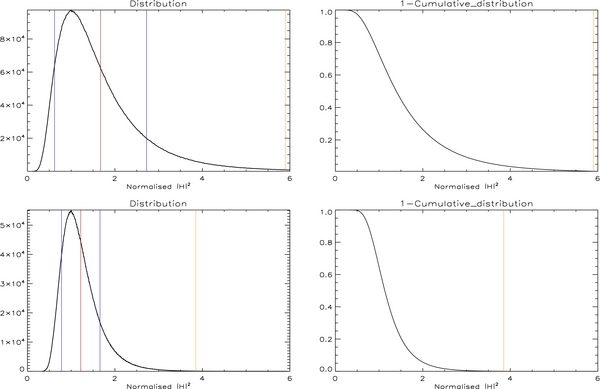
Figure 13. Top row: distribution of normalized egression power in the quiet Sun data cube. The red line corresponds to the ξ, mean egression power in the data cube. The blue lines show ξ ± σ. The orange line corresponds to the peak value of the non-integrated egression at the location of the flare. Bottom row: distribution of the smoothed egression power in quiet Sun data cube. The red line corresponds to the ξ, mean egression power in the data cube. The blue lines show ξ ± σ. The orange line corresponds to the value of the peak in main paper's Figure 10.
Download figure:
Standard image High-resolution imageIf, for the sake of argument, we assume that there are no sources present in the quiet Sun data, and the quiet Sun egression rather ideally represents noise, then the cumulative distribution can be taken as a rough approximation of the probability density function for the egression noise at an individual pixel at any given time in the series. On the other hand, as turbulent convection is considered to be the main method driving acoustic oscillations, it is clear that in all likelihood there will also be real physical sources driving solar oscillations in the observed region. It follows that we can use the quiet Sun cumulative distribution as a rough upper bound estimate on the noise of the method.
Since we use the integrated rms plot as means of distinguishing between spurious peaks and potential acoustic sources, we proceed by computing the smoothed egression power snapshot. This is done by evaluating the integral over a spatial region centered at each point of an egression snapshot. We use a rectangle with the same dimensions as the one used for Figure 10. The distribution and complementary cumulative distribution functions for the smoothed egression power obtained in this way are presented in bottom row Figure 13. It is clear that such smoothing has significantly reduced the width of the distribution indicating the canceling of noise component in the egression measurements.
A.1. Statistical Analysis of Background Seismic Sources
The size of the rectangular integration box used for Figure 10 is ≈20.6 Mm × 7.5 Mm. The mean value of normalized egression in the figure is around 1.5, which drops to around 1.2 if we eliminate several minutes before and after onset of the flare. The peak power in the plot is at 3.85, which is 2.57 times the mean value or 3.2 times the corrected mean value. Thus, the maximum excursion for the suspected quake source exceeds the corrected mean by a factor of 2.2. When we use a larger integration box (see Figure 14), with dimensions ≈24.4 Mm × 13.1 Mm that roughly corresponds to the dimensions of the box in Donea et al. (2006), these values naturally decrease: the mean is 1.22 for the whole time series and 1.11, when the flare data are removed; the maximum is at 3.03, which is 2.48 times the mean or ≈2.73 times the corrected mean value. This statistic on its own compares well with the similar egression rms plots published in Donea et al. (2006) and Martínez-Oliveros et al. (2008a). The maximum value of non-integrated egression power is around 5.9.
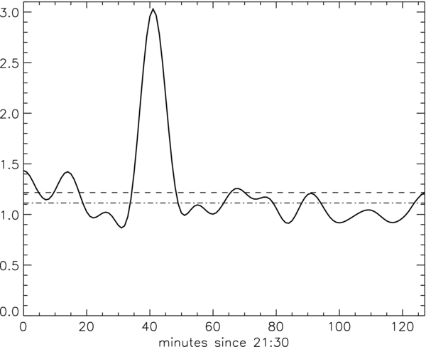
Figure 14. rms plot at the location of acoustic kernels in the flare with integration box dimensions the same as in Donea et al. (2006). The horizontal lines correspond to the means of the series with and without the flare onset data (see the text for more details).
Download figure:
Standard image High-resolution imageWe apply the same processing and integration procedures to the quiet Sun data cube as described in Section 3 for the flare in order to investigate the possibility of having similar excursions in a weak magnetic region. Looking at the egression power computed for quiet Sun data cube, there are a few locations with the maximum magnitude values over 5.9 with the probability of seeing such a peak at a particular location at any time at just below 1%. However, when the data are integrated over 500 s as described in Section 3, the number of such peaks drastically decreases because the stochastic noise contribution cancels itself out, as we demonstrate below.
Generally, the egression power averaged over a more compact region undergoes larger statistical fluctuations. For example, we have also evaluated integration/averaging of egression power over circular regions. This consisted of digitizing two circles with the radii of three and four pixels, respectively, which corresponds to the areas 99.4 Mm2 and 176.7 Mm2. The number of regions with the egression power exceeding the mean by a factor of say, 2.2, is several times higher for the smaller circle. Using the complementary cumulative distribution function (1−F(x)), we estimate the probability of the integrated average having excursion over the same 2.2 times the mean egression to be about 0.0863381% for 4 pixel radius circle region of integration, and 0.303949% for 3 pixel radius. Furthermore, in a similar way, we can evaluate the probability of the events above the given egression amplitude to obtain the probability for the non-integrated egression power to be greater than the maximum value achieved by the flare kernel in Figure 7, which turns out to be ≈2.76599%.
We then smooth the computed quiet Sun egression powers by integrating over the rectangular regions used for the two rms plots. For the smaller rectangle (Figure 10), we find several locations within the central quiet Sun area where the peak in the smoothed egression is over 2.56 times the mean value. For the larger rectangle (Figure 15) there are no locations with the peak value exceeding the mean value by factor of 2.48 or higher. If we repeat the probability estimate for the smoothed egression power, the probability that smoothed egression power rises to the peak in Figure 10 is significantly reduced to approach ≈0.047%.

Figure 15. Peak integrated quiet Sun egression power examples, normalized to have mean at unity. The purple line represents 2.57 factor of the mean egression power representing the value of the peak egression power for the flare.
Download figure:
Standard image High-resolution imageA.2. Conclusions
The peak in egression power detected for the flare site is relatively weak and is comparable to peaks seen in the quiet Sun. However, once the egression is integrated over a suitable region around the peak the stochastic noise contribution cancels itself out. Results of our quiet Sun control exercise show that for a smaller integration box, there are just a handful of quiet Sun locations showing statistics comparable to those extracted for the flare. When the integration box is increased to the size comparable to the one already published (Donea et al. 2006), no such quiet Sun locations were detected at all. This of course can be due to chance and further analysis might be necessary.
Nonetheless, as current thinking considers turbulent convection to be the main method of exciting acoustic oscillations, it is reasonable to assume that over the 2 hr of quiet Sun observations used in our analysis, such sources would be present in the region of interest. These, for example, could be sources produced by the solar turbulence in the inter-granular cells and lanes with lifetime of about a day (Deubner et al. 1992; Gizon et al. 2010) and which are easily picked up by the 2 hr data cube. Therefore, it is likely that at least some of the peaks present the quiet Sun egression computation might correspond to such sources. In such a case the probabilities evaluated in the previous section represent an upper bound estimate for potential noise contribution and are shown to be low. On the other hand, the source associated with the flare cannot be attributed to convective turbulence, since it is located inside a sunspot penumbra which is characterized by the strong magnetic field inhibiting such convection. Therefore this gives us reason to believe that this acoustic emission associated with the flare corresponds to sunquakes excited by the processes that occurred during the course of the flare.
Footnotes
- 3
If F(t) is the cumulative distribution function, we call
 , the complementary cumulative distribution function.