


ABSTRACT
We have constructed an extended composite luminosity profile for the Andromeda galaxy, M31, and have decomposed it into three basic luminous structural components: a bulge, a disk, and a halo. The dust-free Spitzer/Infrared Array Camera (IRAC) imaging and extended spatial coverage of ground-based optical imaging and deep star counts allow us to map M31's structure from its center to 22 kpc along the major axis. We apply, and address the limitations of, different decomposition methods for the one-dimensional luminosity profiles and two-dimensional images. These methods include nonlinear least-squares and Bayesian Monte Carlo Markov chain analyses. The basic photometric model for M31 has a Sérsic bulge with shape index n ≃ 2.2 ± .3 and effective radius Re = 1.0 ± 0.2 kpc, and a dust-free exponential disk of scale length Rd = 5.3 ± .5 kpc; the parameter errors reflect the range between different decomposition methods. Despite model covariances, the convergence of solutions based on different methods and current data suggests a stable set of structural parameters. The ellipticities ( = 1 − b/a) of the bulge and the disk from the IRAC image are 0.37 ± 0.03 and 0.73 ± 0.03, respectively. The bulge parameter n is rather insensitive to bandpass effects and its value (2.2) suggests a first rapid formation via mergers followed by secular growth from the disk. The M31 halo has a two-dimensional power-law index ≃ − 2.5 ± 0.2 (or −3.5 in three-dimensional), comparable to that of the Milky Way. We find that the M31 bulge light is mostly dominant over the range Rmin ≲ 1.2 kpc. The disk takes over in the range 1.2 kpc ≲ Rmin ≲ 9 kpc, whereas the halo dominates at Rmin ≳ 9 kpc. The stellar nucleus, bulge, disk, and halo components each contribute roughly 0.05%, 23%, 73%, and 4% of the total light of M31 out to 200 kpc along the minor axis. Nominal errors for the structural parameters of the M31 bulge, disk, and halo amount to 20%. If M31 and the Milky Way are at all typical, faint stellar halos should be routinely detected in galaxy surveys reaching below μi ≃ 27 mag arcsec−2. We stress that our results rely on this photometric analysis alone. Structural parameters may change when other fundamental constraints, such as those provided by abundance gradients and stellar kinematics, are considered simultaneously.
Export citation and abstract BibTeX RIS
1. INTRODUCTION
Thanks largely to its proximity and kinship with the Milky Way, the Andromeda galaxy, M31, has been the focus of numerous investigations of galaxy structure. Its visual appearance suggests the existence of at least two components within the optical radius: a central bulge and a disk. However, the very faint extended structure around M31 (Ibata et al. 2004, 2007; Guhathakurta et al. 2005, hereafter Guha05; Irwin et al. 2005, hereafter Irwin05; Chapman et al. 2006; Gilbert et al. 2007, 2009b; McConnachie et al. 2009; Tanaka et al. 2010) revealed a complex portrait of galaxy structure that deviates considerably from the original picture of a smooth two-component model for M31. Furthermore, the high-resolution imaging with the Hubble Space Telescope (HST)/WFPC1-2 also shows the existence of a small double-peaked nucleus (Lauer et al. 1993, 1998; Kormendy & Bender 1999, hereafter KB99). Early measurements of M31's luminosity profile from photo-electric photometry (de Vaucouleurs 1958), photographic plates (Walterbos & Kennicutt 1988), and heterogeneous digital imaging and star counts (Pritchet & van den Bergh 1994, hereafter PvdB94) suggested a dominant de Vaucouleurs (1948) profile for M31's bulge. This impression was reinforced by the deep star counts along the minor axis of M31 (Irwin05), which yielded brightness profiles in Johnson-V and Gunn-i bands below 31 and 29 mag arcsec−2, respectively. Irwin05 suggested that a single de Vaucouleurs profile reproduced the minor-axis light of M31 within 1 4 or 19.2 kpc. They also noted (though did not model) that the light profile between 01–04 called for the presence of a faint inner disk.
The rigorous decomposition of structural components in galaxies is critical to our understanding of their formation and evolution. For instance, whether a galaxy surface density profile closely resembles a pure exponential disk (Freeman 1970) or a de Vaucouleurs profile is either indicative of a quiet recent history (e.g., Toth & Ostriker 1992) or a turbulent past (e.g., Bournaud et al. 2007).
In this paper, we examine the luminosity distribution of M31 based on ground- and space-based images and explore the limitations of the various methods that are normally used to extract structural parameters from one-dimensional (1D) brightness profiles and two-dimensional (2D) galaxy images. We model the stellar components of M31 as the sum of a Sérsic (1968) bulge, an exponential disk, and a halo. Despite the limitations of the different modeling procedures, we are able to determine the structural parameters for the main stellar components of M31 with reasonable accuracy.
We present in Section 2 the surface brightness (SB) profiles and star counts from different sources for M31. These will be combined into a single, extended composite luminosity profile for decomposition into various structural components. We discuss in Section 3 the various parameterizations that are most commonly used for decomposition of the 1D and 2D light distributions of the bulge, disk, and halo components in galaxies. Basic 1D and 2D bulge–disk decomposition methods are introduced in Section 4 and model results are compared in Section 5. The effect of a halo component is presented in Section 6, where we analyze the extended composite light profile of M31. We compare in Section 7 our results for the structural parameters for the bulge, disk, and halo of M31 with those from the literature. We conclude in Section 8 with various interpretations of our results and reflect on future decompositions of the M31 structure based on photometric as well as spectroscopic information. Throughout this paper, we adopt a distance DM31 = 785 ± 25 kpc (McConnachie et al. 2005). Thus, at M31, 1'' = 0.0038 kpc (1° = 13.7 kpc). To avoid confusion, all radii labeled "R" refer to a radius measured along the major axis of the galaxy; radii measured along the minor axis of the galaxy are specifically labelled as "Rmin."
2. MEASUREMENTS OF M31'S LUMINOSITY DISTRIBUTION
2.1. Surface Brightness Profiles
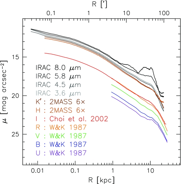
The library of SB profiles for M31 is vast. Table 1 presents a list of the major photographic and digital databases for luminosity profiles and star counts of M31. The SB profiles extracted along the major axis from the galaxy images listed in Table 1 are shown in Figure 1 (star counts are presented in Figure 5).

Figure 1. Azimuthally averaged surface brightness profiles along the major axis for M31. The UBVR profiles were extracted from photographic plates by Walterbos & Kennicutt (1987). The I-band, 2MASS 6X H, K', and IRAC surface brightness profiles were extracted by us from the composite images of Choi et al. (2002), Beaton et al. (2007), and Barmby et al. (2006), respectively.
Download figure:
Standard image High-resolution imageTable 1. Sources of Surface Brightness Profiles for M31
| Reference | Bands | Pixel Scale | Minimum Experiment Time |
|---|---|---|---|
| Walterbos & Kennicutt (1987) | UBVR | Photographic plate | 300–7200 s |
| Pritchet & van den Bergh (1994) | V | Star counts | 2700 s |
| Choi et al. (2002) | I | 2 03 pixel−1 03 pixel−1 |
2400 s |
| Irwin et al. (2005) | Gunn i | Star counts | 800–1000 s |
| Beaton et al. (2007) 2MASS 6X | JHK | 100 pixel−1 |
46.8 s |
| Barmby et al. (2006) IRAC | 3.6 μm, 4.5 μm | 0863 pixel−1 |
62–107 s |
| Gilbert et al. (2009) | V | Spectroscopic star counts | 3600 s |
Download table as: ASCIITypeset image
The much-cited library of UBVR luminosity profiles of M31 from photographic plates by Walterbos & Kennicutt (1987) already highlights the so-called "10 kpc arm," a noticeable bump above a rather exponential disk profile. However, these optical light profiles do not sample the galaxy center well; the starlight in the UBV filters is also sensitive to dust extinction and mostly dominated by bright massive stars, which contribute only a small fraction of the total galaxy stellar mass. KB99 combined and analyzed various V-band light profiles of M31. However, we focus here on redder, less extinction-prone and more spatially extended luminosity profiles.
Choi et al. (2002, hereafter Choi02) derived 17 × 5° B- and I-band CCD mosaics of M31, including M32 and NGC 205, with the Kitt Peak National Observatory Burrell Schmidt telescope. Each mosaic included 35 fields, with a typical exposure time of 40 minutes per field in I. An azimuthally averaged SB profile of this I-band mosaic was extracted via isophotal fitting by Worthey et al. (2005); see the red line in Figure 1. For the purpose of the current analysis, we used the same I-band mosaic from Choi02 to extract a revised I-band azimuthally averaged SB profile as well as I-band major- and minor-axis wedge cuts (see Section 2.2). We reassessed the absolute calibration of the Choi02 data by performing aperture photometry of field stars in that mosaic and adjusting the stellar magnitudes to those computed by the Sloan Digital Sky Survey (SDSS). We used the same point-spread function fitting routines for the Choi02 and SDSS star fields. This procedure yielded a photometric accuracy of ∼0.1 mag (McDonald et al. 2009, hereafter McD09). The calibration from SDSS stars led to a readjustment of 0.4 mag from the photometry reported in Worthey et al. (2005).
Figure 1 shows that the Choi02 data extend as far as the Walterbos & Kennicutt (1987) profiles and better sample the central regions. For this reason, and because the rest-frame I band is a better tracer of the stellar mass than UBV, we use the Choi02 data as our principal anchor for the derivation of a composite light profile for M31. While it would be desirable to combine the data presented in Table 1 into one global composite profile, color gradients thwart that project. Different bands yield different structural parameters, owing to differently distributed stellar populations and dust, selective dust extinction, etc.
High-resolution, wide-field infrared mosaics of M31 remain scant due to the smaller size and lower efficiency of IR arrays, as compared to optical CCDs, and the significant complications due to the rapidly varying infrared sky background. Existing infrared maps come from the Two Micron All Sky Survey (2MASS) 6X survey (Beaton et al. 2007) and the Spitzer Infrared Array Camera (IRAC) survey (Barmby et al. 2006). Beaton et al. (2007) produced a 2.8 deg2 JHK map of M31 as part of the 2MASS 6X program.8 The exposure time per source is six times that of the nominal 2MASS integration, or six times 1.3 s per frame times six frames per source, that is, 46.8 s per source. We have extracted near-IR SB profiles from the 2MASS 6X JHK mosaics according to standard surface photometry techniques (e.g., Courteau 1996; McD09). Counts were calibrated to magnitudes using 2MASS background stars. SB levels were inferred from the 2MASS 6X images using the following transformation: SB[mag arcsec−2] = −2.5log (I[counts]) + z.p., where the zero points are J:22.81, H:22.35, and K:21.85 mag arcsec−2. The H- and K'-band 2MASS 6X azimuthally averaged SB profiles are reported in Figure 1 as brown lines. The 2MASS data (both LGA and 6X) remain ill-constrained beyond the 10 kpc arm due to uncertain sky subtraction (Barmby et al. 2006). Indeed, while the proximity of M31 enables a sharper view of its stellar content, its large apparent size is detrimental for the reliable measurement of the sky level far from the galaxy on timescales shorter than those of the natural fluctuations of the IR sky. Producing an accurately sky-subtracted image for M31 is an extremely challenging task that we address in a forthcoming publication (J. Sick et al. 2011, in preparation). We therefore leave out the 2MASS data from our analysis.
The Spitzer mosaic of Barmby et al. (2006) covers 37 × 16 in the four IRAC bands at 3.6, 4.5, 5.8, and 8 μm. These mosaics sample the galaxy light with 0861 pixels from the center out to the "10 kpc" arm. The integration times per pixel ranged from 62 s in the disk to 107 s in the outskirts. Our extracted IRAC azimuthally averaged SB profiles are shown as gray-to-black lines in Figure 1. For our study, we discarded the 5.8 and 8 μm profiles which are spoiled by polycyclic aromatic hydrocarbon (PAH) emission, especially near the 10 kpc arm. The stellar light at 3.6 and 4.5 μm bands is significantly less contaminated by hot dust features. For simplicity, we only used the 3.6 μm band for our analysis; the 3.6 and 4.5 μm data yield similar profile decompositions.
Although the Spitzer/IRAC images do not have the superb resolution of HST, the IRAC luminosity profiles in Figure 1 already show the suggestive signature at R ≲ 15 pc of a nuclear component. We shall address the modeling of the nucleus in Section 3.1.
It is interesting to note that the signature of the 10 kpc arm shifts inward as a function of wavelength. This is expected if the blue stars lie at the front of the spiral density wave where they were formed; the dust (e.g., PAHs) that results from the evolution of those massive stars will naturally drift behind the stellar front, as observed clearly in the brightness enhancement between 5 and 9 kpc of the IRAC 5.8/8.0 μm light profiles in Figure 1.
2.2. Logarithmic Wedge Profiles
The luminosity profiles shown in Figure 1 are all extracted from azimuthally averaged isophotal fits. However, as with most other spiral galaxies, the light of M31 is a superposition of multiple components with different ellipticities. Isophotal fitting software packages, originally designed for single-component elliptical systems,9 average out the ellipticity information of a galaxy at each pixel such that the fitted ellipses no longer represent one independent structure. This is perhaps the major drawback of profile decompositions based on azimuthally averaged luminosity profiles.
Fortunately, for the case of M31, the position angles of the bulge and disk are within 20° of each other, which lessens the mismatch of superimposed isophotes. However, the ellipticities of the two components are still quite different (see Section 7). Consequently, we shall also explore 1D profile decompositions based on the simultaneous modeling of minor- and major-axis wedge cuts. Such cuts then allow for the modeling of independent galaxian structures. We construct wedge cuts at different azimuthal angles as follows. In order to keep a high signal-to-noise ratio along the cut, we adopted square bins with variable width, W, given by

where n is the bin number, p is the minimum number of pixels at small radius, and N is a constant. The opening angle of the wedge is thus a nonlinear function of galactocentric radius. We have used p = 3 and N = 25.
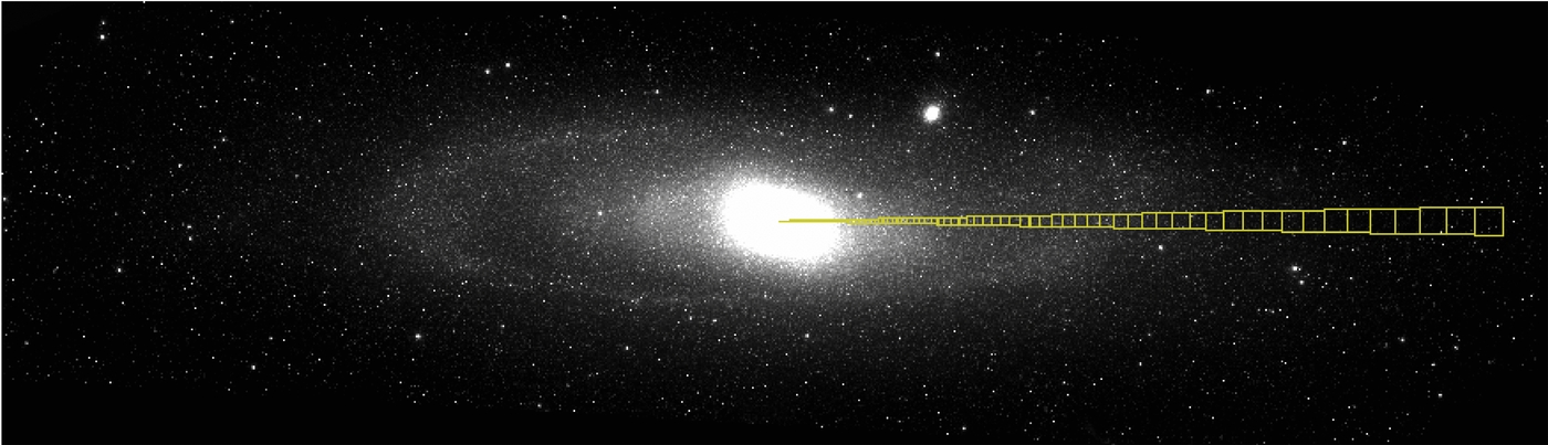
Figure 2 shows the position of the major-axis wedge onto the IRAC 3.6 μm image. A median SB is calculated in each variable-width bin. To remove bright stars, all pixel fluxes more than 3σ above this value are excised and the SB profile is recomputed.

Figure 2. Logarithmic wedge cut (described in Section 2.2), superimposed on the IRAC 3.6 μm image of M31. Each square represents a single bin.
Download figure:
Standard image High-resolution imageThe minor- and major-axis wedge cuts extracted from the Choi02 and IRAC 3.6 μm images are shown in Figure 3. The major-axis cuts are also compared with the azimuthally averaged SB profiles at the I band and at 3.6 μm. Despite our concerns that azimuthal averaging yields, in principle, an unrepresentative blend of distinct luminous components each with different ellipticities, the azimuthally averaged profiles for M31 differ only slightly from the precise cuts. The cuts and averaged profiles are thus interchangeable but the latter have higher signal-to-noise levels.

Figure 3. Minor (upper panel) and major (lower panel) axis brightness profiles for M31, at the I band (blue squares) and IRAC 3.6 μm bands (gray and black circles), as described in Section 2.2. For comparison, our azimuthally averaged profiles for the Choi02 and IRAC 3.6 μm data are shown in red.
Download figure:
Standard image High-resolution imageSubtraction of the I-band and 3.6 μ cuts in Figure 3 reveals color gradients in the inner parts (Rmaj < 20 kpc) of M31. These gradients, shown in Figure 4, are consistent with the bulge being generally populated by more metal-rich stars than the disk, as is seen in other Sb–Sc-like galaxies (MacArthur et al. 2004, 2009; Moorthy & Holtzman 2006; Roediger et al. 2011). The bluing of the disk, especially beyond the 10 kpc ring, confirms that the I-band and 3.6 μm luminosity profiles cannot simply be merged (without corrections) to build an extended composite light profile for M31.

Figure 4. I–3.6 μm color gradients from wedge cuts along the major (left) and minor (right) axes of M31. The color gradient from the azimuthally averaged surface brightness profile (projected along the major axis) is shown as the solid line on the left side. The strong gradient (∼0.5 mag arcsec−2 over the 90' extent of the major axis) is a clear indication that the I-band and IRAC luminosity profiles cannot be merged without radially dependent color corrections. Note the clear bulge–disk transition at roughly 8–10 kpc. Both the M31 bulge and disk get bluer with radius, though at different rates.
Download figure:
Standard image High-resolution image2.3. Profile Error Bars
Rigorous error bars are crucial to the proper model decomposition of a luminosity profile. For azimuthally averaged SB profiles, the quoted intensity per radial increment (here, per pixel) is the median of all the pixel intensities along a given elliptical isophote (light contour) and the brightness error per radial bin is the standard deviation of all those pixel intensities along the isophote with respect to the median intensity value (Courteau 1996). For a wedge cut along any radius, the median intensity per bin is computed as in Section 2.2; the quoted error is the rms deviation about the median value of the pixels in each bin. The latter error estimates can never be an exact representation of the true galaxian (sky-subtracted) photon noise at each bin since each pixel element is smaller than the seeing disk, and all adjacent pixels are thus correlated. The size of the error bars per bin is, however, comparable to the amplitude of the point-by-point fluctuations (see Figure 3), suggesting that our error estimates are reasonable.
The error bars as quoted by the authors for the Irwin05 profiles are significantly larger, at large radii, than the point-by-point fluctuations. For our modeling of the Irwin05 data, we have recomputed those errors as the standard deviation about linear fits through neighboring data points. These errors closely reflect the point-by-point fluctuations of the data.
2.4. Star Counts
In addition to the galaxy images and surface brightness profiles, information about the shape of the galaxy components can be gleaned from star counts measured in fields around the disk of the galaxy where crowding effects are lessened. We have combined the extended star counts of the M31 stellar halo largely along the minor axis by PvdB94, Irwin05, and Gilbert et al. (2009a, hereafter G09). These star counts cover the range 20 kpc ⩽Rmin ⩽ 150 kpc (along the minor axis; see also Ibata et al. 2007; McConnachie et al. 2009).
PvdB94 obtained digital star counts with the Canada–France–Hawaii Telescope in the V band for eight fields along M31's minor axis. Each field was observed three times for a minimum of 900 s per integration. These counts were then combined with photographic luminosity profiles by de Vaucouleurs (1958) and Walterbos & Kennicutt (1987) and digital imaging by Kent (1983). The PvdB94 minor-axis brightness profile is shown with red circles in Figure 5. Based on these data, PvdB94 postulated that the halo of M31 along the minor axis was well represented by a single de Vaucouleurs law over the range 0.2 kpc ⩽Rmin ⩽ 20 kpc.

Figure 5. Composite minor-axis profile, described in Section 2.4. The radius is projected along the minor axis. The I-band minor-axis brightnesses, shown in blue, were extracted from the I-band image of Choi et al. (Choi02). Extension of the Choi02 profile relies on the star counts of the M31 stellar halo largely along the minor axis by Irwin et al. (Irwin05) in green, Pritchet & van den Bergh (PvdB94) in red, and Gilbert et al. (G09) shown in black. The Irwin05 error bars were re-derived by us (Section 2.3).
Download figure:
Standard image High-resolution imageIrwin05 used stellar counts from the Isaac Newton Telescope to determine M31's luminosity profile along its southeast minor axis. They combined PvdB94's data with faint red giant branch star counts to trace the minor-axis stellar distribution out to a projected radius of ∼55 kpc, where μV ∼ 32 mag arcsec−2. They exposed typically 800–1000 s per field per bandpass in Johnson V and Gunn i. We show their Gunn-i minor-axis luminosity profile as green dots in Figure 5. Irwin05's analysis corroborated PvdB94 with a de Vaucouleurs profile out to a projected minor-axis radius of ∼20 kpc. Beyond that radius, Irwin05 surmised, the light profile would assume a more exponential shape with a scale length of 14 kpc. We will see in Section 6 that the M31 minor-axis cut is indeed a poor tracer of disk light. Indeed, our decompositions argue against a de Vaucouleurs profile (Sérsic n = 4) for the M31 bulge.
Guha05 presented a V-band SB profile along M31's southeastern minor axis based on counts of resolved member red giant stars in a Keck/DEIMOS spectroscopic survey. The spectroscopic exposure time with Keck/DEIMOS was 1 hr per field. Red giants in M31 were identified (and distinguished from foreground Milky Way dwarf star contaminants) using a combination of photometric and spectroscopic diagnostics (Guhathakurta et al. 2006; Gilbert et al. 2006). To estimate M31's stellar surface density as a function of radius, the observed ratio of M31 red giants to Milky Way dwarf stars was multiplied by the surface density of Milky Way dwarf stars predicted by the "Besançon" Galactic star-count model (e.g., Robin et al. 2003, 2004). This estimate was then calibrated to the V-band intensity by comparing it with the PvdB94 data in overlapping regions (also based on star counts). The minor-axis SB profile from V-band counts, presented here as black dots in Figure 5, includes two improvements relative to the Guha05 analysis—as reported in G09: (1) a larger number and wider spatial distribution of Keck/DEIMOS spectroscopic fields providing denser sampling over the radial range 10 < R < 165 kpc (Kalirai et al. 2006; Gilbert et al. 2007), and (2) correction for field-to-field variations in the spectroscopic sample selection function.
2.5. Composite Minor-axis Profile
The extended minor-axis composite profile of M31 shown in Figure 5 is a combination of the minor-axis wedge cut from the image of Choi02 (Section 2.2) and the deep minor-axis star counts of Irwin05, PvdB94, and G09. The star counts were all normalized to our recalibrated I-band profile for Choi02. Altogether, our composite profile yields a detailed picture of M31's global I-band luminosity distribution for μI < 30 mag arcsec−2. Figure 5 may be compared, for Rminor < 80 kpc, with Figure 31 of Ibata et al. (2007), using V − I ∼ 2.
Our modeling of the composite profile can either treat all the data points independently ("Unbinned") or use a uniformly sampled profile that has been averaged over all overlapping data ("Binned"). Both techniques are often found in the literature and we wish to test them here. A weighted fit should in principle yield similar solutions for both the unbinned and binned profiles since the former will have more data points per bin (in regions of data overlap) while the latter will have, on average, smaller error bars per bin. Reality is not always so simple.
In order to create a single, composite, "binned" minor-axis profile from the four above-mentioned profiles, we adopted a logarithmic binning as in Equation (1) with p = 3 and N = 25. These parameters were chosen to match the inner regions of the I-band profile minor-axis profile. The surface brightness per bin is the error-weighted average of the surface brightnesses from all of the available data in that bin. The error per bin is the root-mean-square of all the data point errors in that bin. We will analyze both the unbinned and binned composite profiles in Section 7.
3. GALAXY MODEL COMPONENTS
We decompose the M31 1D luminosity distribution and 2D image into basic galaxy model components. Visual examination of Figures 1 and 5 suggests the existence of at least four distinct stellar components in M31: a nucleus, a bulge, a disk, and a halo.
The 1D luminosity profiles for our bulge and disk (hereafter B/D) decompositions without a halo component consist of the I-band and IRAC 3.6 μm azimuthally averaged (hereafter "AZAV") SB profiles (Figure 1) and major- and minor-axis cuts (Figure 3). As seen in these figures, the profiles extend out to roughly 6 kpc along the minor axis or 23 kpc along the major axis. We use the I-band composite minor-axis profile (Figure 5), which now extends out to 200 kpc along the minor axis, for decompositions that include a halo component. We also use the IRAC 3.6 μm image to derive a model decomposition of the 2D light distribution within 23 kpc using the GALFIT program of Peng et al. (2002, hereafter GALFIT). The IRAC image is preferred for 2D modeling to that of Choi02 for its higher resolution, lesser sensitivity to dust, and comparable spatial extent. However, given its relatively shallow depth, the IRAC image of M31 cannot be used to model the halo component.
We now discuss the galaxy model component parameterizations. Except for the nucleus, seeing convolution of the model functions is unnecessary for the nearby M31.
3.1. Galaxy Nucleus
As noted above, Lauer et al. (1993) were first to show with their HST/WFPC1 images that the M31 nucleus was double-peaked. Despite the poorer resolution of our IRAC images, and our inability to resolve two distinct sources, the gentle central rise of the IRAC light profiles for R < 15 pc in Figure 1 is clearly suggestive of a nucleus component. KB99 used Lauer's HST/WFPC1-2 images of the M31 core and high spatial-resolution CFHT/SIS spectra to infer that the M31 nucleus is a separate component with an origin different from that of the bulge. The well-resolved HST V-band images analyzed by KB99 show a nearly exponential nucleus (see Equation (4) below) with a scale length Rn = 088 = 3.3 pc (J. Kormendy 2011, private communication). The nucleus contributes only a very small fraction (<0.05%) of M31's total luminosity budget. M31's nucleus is indeed sufficiently small that the model parameters for the bulge, disk, and halo are largely unaffected by it. Therefore, while we embrace the results by Lauer et al. (1993) and KB99, we now ignore the nucleus component in our luminosity profile decompositions.
3.2. Galaxy Bulge
We assume that the 2D luminosity distribution of the M31 bulge has a projected profile given by the Sérsic (1968) profile,

where Re is the projected half-light radius, Ie is the intensity at Re, the exponent n is the Sérsic shape parameter, and bn = 1.9992n − 0.3271 (Capaccioli 1989). With n = 1 or n = 4, the Sérsic function reduces to the exponential or de Vaucouleurs functions, respectively.
The total extrapolated luminosity of a Sérsic bulge is given by

where a and b are the semimajor and semiminor axes of the bulge. We will use Equation (3) to compute the bulge total light fraction in Section 7. See Graham & Driver (2005) for more details about the Sérsic function.
3.3. Galaxy Disk
We assume that the projected light profile of the disk is described by a basic exponential function,

where I0 is the disk central intensity and Rd is the projected disk scale length. The total extrapolated luminosity of an exponential disk is given by

where a and b are now the semimajor and semiminor axes of the disk.
Various authors (Kormendy 1977; Baggett et al. 1998; Puglielli et al. 2010) have considered an inner disk truncation as an alternative to modeling galaxy light profiles with a dip at the bulge–disk transition. Such a dip can be understood through various effects, such as dust extinction (MacArthur et al. 2003, hereafter Mac03) or the mixing action of a dynamical hot stellar bulge or bar (Puglielli et al. 2010). However, we ignore the possibility of a core in the inner disk of M31, as the current study based on imaging data alone offers no leverage for testing this hypothesis. We limit our modeling of the disk to a pure exponential function with a constant scale length at all radii.
3.4. Galaxy Halo
The deep star counts from Irwin05 and G09, shown in Figure 5, are clearly indicative of an additional component at Rmin ≳ 12 kpc, which appears to be independent of the galaxy disk (see also Ibata et al. 2007; Tanaka et al. 2010). As shown by Gilbert et al. (2007, G09), the kinematics of the stars in tidal streams out to 60 kpc show a large spread in velocities, consistent with expectations for a halo population. In Section 7.3, we also suggest that the M31 bulge and halo components are likely independent on account of their different spatial distributions.
We model the (1D) halo with either a Sérsic function (Equation (2)) or a power law:

where R* is a turnover radius and I(R*) = I*. The magnitude formulation is simply μh = −2.5log Ih. Based on visual examination of Figure 5, we adopt R* = 30 kpc (measured along the minor axis) where the halo is dominant. The value of R* is arbitrary and only affects I*. The quantity ah sets the amplitude of the profile in the inner parts. Note that at large radii, the Hernquist model (Hernquist 1990) and the Navarro–Frenk–White (NFW) function (Navarro et al. 1996), as explored for the M31 halo by, e.g., Ibata et al. (2007) and Tanaka et al. (2010), are special cases of our power-law model.
For the power-law halo, the total luminosity is

where a* = ah/R* and smax = Rmax/R*. In this work, we integrate out to a maximum radius Rmax = 200 kpc along the minor axis.
We also assume a spherical halo (a = b) as the current star counts offer no leverage on the halo shape. If M31's halo is anything like the Milky Way's, our assumption of a spherical halo is well justified (Majewski et al. 2003; De Propris et al. 2010; however see Bell et al. 2008).
4. DECOMPOSITION METHODS
To achieve model decompositions of the galaxy's 1D light profiles (azimuthal averages or radial cuts) and 2D image, we use different basic fitting methods based on frequentist or Bayesian methodologies. The 1D azimuthally averaged SB profiles and wedge cuts for M31 can be decomposed into the different model components above using a nonlinear least-squares (hereafter "NLLS") minimization method based on the Levenberg–Marquardt algorithm (downhill gradient). Such a "frequentist" approach for the decomposition of galaxy components has been implemented by many (e.g., Kent 1985; KB99; Mac03; McD09). The robustness of the "NLLS" method is discussed in Mac03. The model parameter 1σ error bars are computed as in Mac03 and McD09. Those errors reflect the 68% range of solutions from a full suite of Monte Carlo NLLS realizations with a complete range of initial guesses over all possible fitted parameters. Because the adopted structural models are usually not ideal representations of the real structure of a galaxy, the statistical errors per model parameter from NLLS fitting codes are usually rather small, much more so than the errors computed through the Monte Carlo method alluded to above.
An alternative approach is to implement Bayesian statistics and a Markov Chain Monte Carlo (hereafter "MCMC") analysis. The aim here is to determine the posterior probability, P(M|D, I), that is, the probability of the model, M, given the data, D, and prior information, I. Since our model is expressed in terms of a set of parameters, P(M|D) takes the form of a probability distribution function (pdf) over the model parameter space. The calculation is performed via Bayes' theorem, which states that P(M|D, I)∝P(M)P(D|M), where P(D|M) is the probability of the data given the model, and P(M) is the prior probability on the model parameters. In fact, P(D|M) is the likelihood function of the NLLS method described above. The Bayesian approach is more ambitious. With NLLS, one is simply interested in the values of the parameters that maximize the likelihood function. Here, one must calculate (or at least estimate) P(M|D, I) as defined over the entire model parameter space.
In principle, Bayesian inference provides a more complete understanding of how well the model describes the data (the state of our knowledge). For example, one can calculate the pdf for any set of quantities (say, a subset of the model parameters or quantities derived from the model parameters) by integrating P(M|D, I) over the parameter space (marginalization). In this way, one can obtain confidence limits on the parameters. By contrast, with NLLS, confidence limits on the parameters are obtained from the shape of the likelihood function near the peak. Now if the likelihood function is single-peaked and well behaved, and if our prior, P(M), is relatively constant over the range where P(M|D, I) is appreciable, then the peak in P(M|D, I) will be very close to the parameter values obtained by simply maximizing P(D|M) (though again, we stress that the calculation and interpretation of the confidence limits is different for the two methods). For a review of Bayesian inference and how it compares with the frequentist approach, see Gregory (2005).
Calculation of P(M|D) often involves complicated, multi-dimensional integrals. For example, in the case where we include a bulge, disk, and halo component, and consider both major- and minor-axis profiles (and hence require ellipticities for the three components), the model is described by 10 parameters making a direct calculation (or, for that matter, a grid search in a maximum-likelihood scheme) prohibitively time-consuming. Hence, we resort to the powerful MCMC method. With MCMC, P(M|D, I) is approximated by a chain of points in the parameter space which is constructed via a simple set of rules. In our work, we employ the Metropolis–Hastings algorithm (Metropolis et al. 1953; Hastings 1970). For a chain of sufficient length, the distribution of points along the chain is the pdf, P(M|D). Pdfs for any subset of parameters are obtained by simply projecting the chain onto the appropriate subspace.
The Metropolis–Hastings algorithm is described in numerous documents. The engine of the algorithm is the jumping rule, which must be chosen with care in order to ensure that the Markov chain adequately approximates P(M|D, I). In this paper, we use an iterative scheme which is similar to simulated annealing (see Puglielli et al. 2010).
For the present analysis, we choose a uniform prior for the scale-free parameters (e.g., μd, ) and a logarithmic, or Jeffrey's prior (equal probability per decade), for the scaling parameters (e.g., Rd, Re). In addition, we introduce a "noise" parameter for each data set. That is, the likelihood function, P(D|M), is taken to be

where σ2ij = eij2 + f2j. In these expressions, j denotes the different data sets (IRAC, Choi02, etc.) while i labels the data points within each data set. The noise parameters fj can account for features in the data not explained by the model or for the possibility that the quoted measurement errors eij were underestimated. The noise parameters are included in the model parameter space with a Jeffrey's prior. For the calculation, we treat all quantities in counts. However, the noise parameter is taken to be a fractional error, i.e., fj = sjdij, so the actual parameter in the MCMC analysis is sj.
We can also decompose 2D galaxy images using similar parameterizations as for the 1D case, through the simultaneous matching of the image pixel distribution by a 2D model, using a downhill gradient algorithm. Much like the simultaneous analysis of 1D profile cuts taken at different position angles (hereafter P.A.'s), the 2D multi-component fitting enables the determination of distinct ellipticities for the underlying galaxy components. Unlike our 1D isophotal maps, the 2D models assume a constant ellipticity and P.A. for each axisymmetric component. For the fitting of 2D parameterized, axisymmetric, functions to astronomical images, we here adopt the (frequentist) GALFIT galaxy/point source fitting algorithm by Peng et al. (2002).
To assess the robustness of the 2D fits and the sensitivity of the final 2D galaxy model to the initial guesses, we have performed a suite of decompositions with initial guesses spanning a wide range of values. The initial guesses for the geometrical parameters (P.A. and axial ratio) were set according to the best 1D isophotal fits. We find the 2D decompositions to be rather insensitive to deviations of the initial guesses, with final best-fit parameters differing by no more than 0.1%. Much like the 1D NLLS error analysis, the 1σ error estimate per fitted parameter reflects the small range of GALFIT solutions for a broad range of initial guesses.
We have also tested for the effect of sky uncertainties. In the 1D analysis, using the Choi02 image, we computed model parameters based on sky levels that differ by 1σ from the mean. That sigma was determined from the standard deviation of sky levels measured in five sky boxes adjacent to the galaxy. With those different sky levels, the scale radii and bulge n can vary by no more than 7%–9% and the effective surface brightnesses by less than one-tenth of a magnitude. Similar results apply for our 2D image. For the latter, we have also tested for a floating sky in GALFIT. This results in a 0.6% decrease in the bulge scale length and 1.3% decrease in the disk scale length. The geometry of the bulge/disk system is unchanged. All cases considered, our results are robust against sky-level uncertainties.
For the 2D fits, we only model the IRAC 3.6 μm image with GALFIT (for reasons explained in Section 3). Also, the latter requires an exposure time map, for the construction of a pixel-to-pixel variance map, which cannot be reconstructed for the Choi02 mosaic. This variance map assumes Poisson statistics, calculated from the coverage maps of the IRAC mosaics. Since the IRAC images are too shallow to reveal the stellar halo component, our GALFIT modeling is limited to a Sérsic bulge and an exponential disk. Each component has its own ellipticity and P.A. The latter is a significant advantage over our implementations of 1D NLLS and MCMC techniques.10
A further complication for GALFIT errors is the issue of SB fluctuations in the outer disk which, for M31, can be large compared to the Poisson noise (owing to the proximity of M31). We have tested for this effect in our construction of the variance map for the 2D fit. Accounting for SB fluctuation errors can alter model parameters by ∼10%. Those are the typical errors that we quote for the model parameters in Table 3. These could be larger on account of other systematic effects that we have not accounted for, such as the modeling of a bar and the effect of a variable tilt in the M31 disk. The random errors are otherwise negligible in light of the very high signal-to-noise ratio of the IRAC 3.6 μm pixels.
The 1D and 2D approaches to modeling galaxy luminosity profiles and images may yield different results due to their intrinsic differences (e.g., different convergence algorithms, weighting schemes, accounting for P.A.'s and ellipticities, etc.11). As we discussed in Section 3, the choice of minimization against counts or magnitudes can potentially yield different solutions. However, we have verified that provided the errors are correctly propagated and given the present data for M31, our minimizations against magnitudes or counts yield similar results.
5. COMPARISON OF METHODS
We first address intrinsic differences between the 1D NLLS and MCMC modeling techniques, as well as against 2D modeling, with a simplified data set and a simple fitting model. To this end, we model only a Sérsic bulge and a disk with the IRAC 3.6 μm and the Choi02 data. The B/D decompositions of the 1D IRAC and Choi02 luminosity profiles from both our NLLS and MCMC methods are reported in Table 2. Decomposition parameters of the 2D IRAC image with GALFIT are presented in Table 3. The B/D parameters in Tables 2 and 3 correspond to the parameters in Equations (2) and (4). The surface brightnesses, computed as μ = −2.5log I mag arcsec−2, are not corrected for projection or extinction effects. The B/D ellipticities, bulge = 1 − (b/a)bulge and disk = 1 − (b/a)disk, are presented where available.
Table 2. Bulge/Disk Decompositions for M31
| Model | Data | Method | Cut | n | Re | μe | bulge |
Rd | μ0 | disk |
|---|---|---|---|---|---|---|---|---|---|---|
| (kpc) | (mag arcsec−2) | (kpc) | (mag arcsec−2) | |||||||
| A | IRAC | MCMC | Maj | 2.46 ± 0.09 | 1.09 ± 0.07 | 16.2 ± 0.10 | ... | 5.09 ± 0.17 | 16.83 ± 0.07 | ... |
| B | IRAC | NLLS | Maj | 2.3 ± 0.3 | 1.0 ± 0.2 | 16.1 ± 0.3 | ... | 5.4 ± 0.3 | 16.8 ± 0.1 | ... |
| C | IRAC | MCMC | Min | 2.01 ± 0.11 | 0.53 ± 0.05 | 15.47 ± 0.13 | ... | 1.29 ± 0.09 | 16.49 ± 0.25 | ... |
| D | IRAC | NLLS | Min | 1.9 ± 0.5 | 0.5 ± 0.3 | 15.4 ± 0.5 | ... | 1.3 ± 0.6 | 16.4 ± 15 | ... |
| E | IRAC | MCMC | MinMaj | 2.18 ± 0.06 | 0.82 ± 0.04 | 15.77 ± 0.07 | 0.21 ± 0.01 | 4.71 ± 0.14 | 16.62 ± 0.05 | 0.74 ± 0.01 |
| F | IRAC | NLLS | AZAV | 2.4 ± 0.2 | 1.10 ± 0.10 | 16.1 ± 0.10 | ... | 5.8 ± 0.1 | 16.79 ± 0.02 | 0.74 ± 0.02 |
| G | IRAC | MCMC | AZAV | 1.66 ± 0.03 | 0.68 ± 0.01 | 15.34 ± 0.03 | ... | 4.75 ± 0.01 | 16.41 ± 0.01 | ... |
| H | IRAC | NLLS | AZAVmsk | 2.2 ± 0.3 | 1.00 ± 0.10 | 16.0 ± 0.20 | ... | 4.9 ± 0.1 | 16.70 ± 0.10 | 0.74 ± 0.02 |
| I | Choi02 | MCMC | Maj | 2.06 ± 0.06 | 0.91 ± 0.04 | 18.12 ± 0.08 | ... | 5.69 ± 0.09 | 18.97 ± 0.03 | ... |
| J | Choi02 | NLLS | Maj | 2.2 ± 0.3 | 1.12 ± 0.10 | 17.3 ± 0.2 | ... | 6.4 ± 0.1 | 18.14 ± 0.04 | ... |
| K | Choi02 | MCMC | Min | 1.85 ± 0.07 | 0.51 ± 0.02 | 17.62 ± 0.08 | ... | 1.73 ± 0.05 | 18.99 ± 0.08 | ... |
| L | Choi02 | NLLS | Min | 1.9 ± 0.2 | 0.53 ± 0.03 | 17.7 ± 0.1 | ... | 1.68 ± 0.04 | 18.8 ± 0.1 | ... |
| M | Choi02 | MCMC | MinMaj | 1.83 ± 0.04 | 0.74 ± 0.02 | 17.73 ± 0.05 | 0.28 ± 0.01 | 5.47 ± 0.08 | 18.91 ± 0.03 | 0.70 ± 0.01 |
| N | Choi02 | NLLS | AZAV | 2.00 ± 0.4 | 1.00 ± 0.30 | 18.2 ± 0.4 | ... | 5.80 ± 0.10 | 19.0 ± 0.3 | 0.71 ± 0.02 |
Download table as: ASCIITypeset image
Table 3. GALFIT Bulge/Disk Decompositions of the M31 IRAC 3.6 μ Image (Parameter Errors Are Typically 10%)
| Model | Method | n | Re | μe | bulge |
Rd | μ0 | disk |
|---|---|---|---|---|---|---|---|---|
| (kpc) | (mag arcsec−2) | (kpc) | (mag arcsec−2) | |||||
| O | Original image | 1.9 | 0.9 | 16.1 | 0.37 | 5.9 | 17.1 | 0.72 |
| P | Masked image | 2.0 | 1.0 | 16.2 | 0.37 | 5.9 | 17.1 | 0.72 |
| Q | Forced bulge, disk |
2.1 | 0.9 | 16.9 | 0.21 | 5.7 | 16.8 | 0.74 |
Download table as: ASCIITypeset image
In Table 2, the column "Cut" can have "Min" and "Maj" for independent minor-axis or major-axis cuts, respectively (see Models A–D and I–L). The notation "MinMaj" identifies the simultaneous use of both the minor and major profile cuts with our MCMC code to yield, like GALFIT with a 2D image, independent estimates of the B/D mean ellipticities (see Models E and M). "AZAV" and "AZAVmsk" refer to the azimuthally averaged surface brightness profile, whether raw or with spiral arms clipping, respectively (Models F–H and N). Spiral arms clipping for surface brightness profiles is discussed in McD09; it is meant to exclude the portion of the profile that is affected by a spiral arm, revealing the underlying exponential stellar profile (an alternative approach is also to fit, rather than clip, the spiral arm features. This approach introduces additional parameter covariance). A natural consequence of azimuthal averaging is that (non-circular) arms appear broader in AZAV profiles than they do along any azimuthal cut. A thin, logarithmic spiral arm can project into a wide azimuthally averaged feature in a 1D AZAV profile, giving the illusion of a broader arm (or bar). Spiral arm clipping thus removes more bona fide old disk light in 1D than it would in 2D with a non-axisymmetric model of the arms.
Note that the structural parameters listed in Table 2 for "Min" cuts are those projected along the minor axis of M31, while those listed for the "Maj," "MinMaj," or "AZAV" profiles refer to projection along the major axis of M31.
While our NLLS algorithm was not coded to extract ellipticities from cuts of different P.A.'s, the isophotal fits of the IRAC and Choi02 images yield ellipticity profiles that can be compared to the MCMC values for bulge and disk. The disk ellipticities from both isophotal fitting and the MCMC analysis are identical; these are not affected by the presence of a bulge. The bulge ellipticity, bulge, cannot be estimated from isophotal fits since the inner ellipticities are the result of superimposed structural components. We return to the comparison of 1D and 2D ellipticities in Section 7.
Given the same data and fitted models, as in Models A–D, F–G, and I–L, the NLLS and MCMC methods are nearly equivalent; some differences exist (e.g., Models F and G) largely due to operational differences between the NLLS and MCMC methods. Models F and G treat AZAV data that are far better sampled in the outer disk than the Min/Maj cuts for Models A–D and I–L. The sensitivity to the 10 kpc arm is thus enhanced in the AZAV profile, via smaller error bars per point. In Model G, the Bayesian MCMC analysis includes a "noise" parameter which is added, in quadrature, to the calculated error. This parameter effectively softens the impact of non-exponential spiral disk features. The net result is a fit that does worse, relative to F, in the center but slightly better at large radii. Effectively, MCMC ignores the "10 kpc" arm signature in the SB profile while NLLS (as coded) must force a fit. This is made even more evident when the spiral arms are masked in Model H; the disk structural parameters come to a closer agreement with the MCMC Model G. The conservative conclusion for Model G is that it yields a lower limit on the range of allowed values of n for the M31 bulge. Figure 6 also shows that the MCMC Model E and the NLLS Model H (with masked spiral arms) yield virtually identical results.

Figure 6. Left: MCMC decomposition of the IRAC 3.6 μm minor- and major-axis cuts for M31 with a Sérsic bulge and an exponential disk model. The squares show the major-axis cut and the dashed lines are the fitted bulge and disk component of Model E in Table 2. The spike near the center (R ∼ 0) in the data-model residuals (bottom panel) is due to the nucleus. Right: NLLS decomposition of the IRAC 3.6 μm azimuthally averaged surface brightness profile (with masked arms), here shown with black crosses, with a Sérsic bulge and an exponential disk model from Model H in Table 2. The data-model residuals are also shown in the bottom panel. Despite using two different decomposition methods, Models E and H are virtually identical (within the errors).
Download figure:
Standard image High-resolution imageThe 1D B/D decompositions from Table 2 (Models A–H) can be compared with our GALFIT B/D analysis of the 2D IRAC 3.6 μm image. Results from the latter are reported in Table 3. We have explored the effect of spiral arm clipping (Models O versus P) but the differences are minimal. This result may seem surprising in light of the contrast between Models F and H, but recall that the spiral arms are less dominant in the 2D image. Unlike in 1D, the 2D fitting technique primarily picks out and fits the axisymmetric features in the data, and thus the non-axisymmetric spiral arms have less influence in 2D than in 1D. Indeed, unlike the variations between the NLLS Models F and G, the comparison of GALFIT Models O and P here shows little difference with arm masking.
We also explore in Model Q, which is unmasked, a forced GALFIT decomposition with B/D ellipticities for our 1D model decomposition E to test whether the 1D and 2D solutions differ only by virtue of their separate ellipticity and P.A. values. The GALFIT parameters with variable (Model O) or forced (Model Q) ellipticity certainly differ in the sense that the 2D (NLLS) Model Q approaches the 1D (NLLS) Model F. Some of the differences between Models Q and, say, E, which can be as large as ∼10%–20%, thus stem from using different component orientations (P.A.'s) and ellipticities, providing yet another reason to embrace 2D model decompositions.
Note that the total light fraction of the GALFIT bulge and disk (B/D)-only fit is 29% for the bulge and 71% for the disk. We also compute the total IRAC 3.6 μm flux of M31 as M3.6 = −24.43 or L3.6 = 1.17 × 10¹¹ L☉.
We can summarize the current state of model comparison as (1) for simple data sets, the NLLS and MCMC methods yield comparable results; (2) the MCMC method enables the identification of data-model inadequacies; and (3) structural parameters can change by ∼10%–20% when P.A. and ellipticity differences for the bulge and disk viewed in 1D or 2D are taken into account. Finally, the differences between the 1D B/D decomposition parameters in Table 2 for the 3.6 μm IRAC and I-band Choi02 data are largely due to waveband effects (see Section 7).
6. ANALYSIS OF THE COMPOSITE PROFILE
Having examined the validity of simple B/D model decompositions, we now consider a more elaborate scheme with the decomposition of our 1D I-band composite profile (Figure 5) into three structural components: a bulge, a disk, and a halo. From visual inspection of Figure 5, it is unclear which parameterization best suits the faint data. We only consider here a Sérsic (Equation (2)) or a power-law (Equation (6)) function. The decomposition results are reported in Table 4 for the power-law halo and in Table 5 for the Sérsic halo.
Table 4. I-band Composite; Bulge/Disk/Power-law Faint
| Model | Method | Cut | n | Re, b | μe, b | Rd | μ0 | α | μ* | ah |
|---|---|---|---|---|---|---|---|---|---|---|
| (kpc) | (mag arcsec−2) | (kpc) | (mag arcsec−2) | (mag arcsec−2) | (kpc) | |||||
| R | NLLS | Min/Bin | 2.20+.20−.20 | 0.60+.10−.10 | 17.90+.30−.30 | 1.70+.30−.30 | 18.80+.30−.30 | 1.10+.10−.10 | 27.70+.10−.10 | 11.40+0.10− 0.10 |
| S | MCMC | Min/Bin | 2.67+.11−.11 | 1.77+.05−.05 | 19.53+.07−.07 | 0.12+.02−.02 | 15.60+.20−.20 | 1.78+.29−.30 | 27.90+.08−.08 | 55.65+12.3− 12.6 |
| T | MCMC | Min/UnBin | 1.89+.10−.10 | 0.51+.03−.03 | 17.66+.11−.11 | 1.54+.05−.05 | 18.72+.09−.09 | 1.14+.09−.09 | 28.32+.09−.09 | 6.60+1.22− 1.20 |
| U | MCMC | MinMaj/UnBin | 1.90+.05−.05 | 0.73+.02−.02 | 17.79+.05−.05 | 5.02+.05−.06 | 18.81+.02−.02 | 1.26+.04−.04 | 28.07+.05−.05 | 5.20+0.16− 0.16 |
Download table as: ASCIITypeset image
Table 5. I-band Composite; Bulge/Disk/Sérsic Faint
| Model | Method | Cut | n | Re, b | μe, b | Rd | μ0 | nf | μe, f | Re, f |
|---|---|---|---|---|---|---|---|---|---|---|
| (kpc) | (mag arcsec−2) | (kpc) | (mag arcsec−2) | (mag arcsec−2) | (kpc) | |||||
| V | NLLS | Min/Bin | 2.00+.30−.30 | 0.50+.10−.10 | 17.70+.20−.20 | 1.40+.20−.20 | 18.60+.30−.30 | 4.90+0.80− 0.80 | 24.70+2.0− 2.0 | 9.00+1.3− 1.3 |
| W | MCMC | MinMaj/Unbin | 1.80+.05−.05 | 0.69+.02−.02 | 17.72+.05−.05 | 5.05+.05−.06 | 18.80+.02−.02 | 5.39+0.79− 0.80 | 26.11+.08−.08 | 13.36+0.5− 0.5 |
Download table as: ASCIITypeset image
First, the comparison of Models R and S reminds us of MCMC's ability to compensate for inadequate data-model matching. Contrary to Model R, MCMC's Model S calls for an extended, faint bulge coupled with a very compact, bright disk. The data-model errors or bulge–disk model covariances are sufficiently large as to yield an uncertain decomposition. The disk component is nearly absent in this minor-axis cut decomposition (reminiscent of PvdB94's, Irwin05's, and G09's results). The bulge component absorbs much of the disk contribution, making the bulge completely dominant. The parameters of Model S are also significantly different from those of Models R, T, and U. This situation may have led to the large central n values for the M31 bulge reported in the past. Note that the NLLS approach (Model R) forces a disk solution but the fit parameters are never constrained.
6.1. To Bin or Not to Bin?
We can exploit different modeling techniques through a combination of 1D NLLS and MCMC analysis with "Binned" or "Unbinned" cuts. The "unbinned" method comes from our consideration of all the data points in our four individual cuts (Choi02, Irwin02, PvdB94, and G05) treated individually. The "binned" approach consists of averaging the four data sets into one composite profile; the overlapping data at any given radius are weight-averaged according to their respective errors. The differences in model parameters for the "Binned" versus "Unbinned" data, as seen in the Model pair S/T, can also be rather significant. Unless a precise argument can be made for data binning (e.g., improvements of the signal-to-noise ratio), the latter is best avoided.
6.2. Power-law versus Sérsic Halo
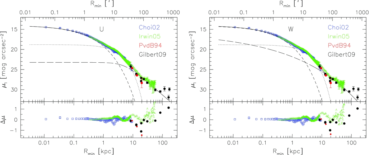
Figure 8 shows the composite profile decompositions with Models U (power law; left) and W (Sérsic; right). Both models look statistically comparable given the similar residual distributions. Based on global χ-square statistics for NLLS Models R and V, which rely on minor-axis data only, and visual impression of the data-model residuals (figure not shown), the power-law fit seems to be a marginally better description of the outer profile of M31.
However, the MCMC "MinMaj" Models U and W, which must also account simultaneously for the major-axis I-band data of Choi02, are intrinsically more rigorous than Models R and V. The probability distributions for the parameters of Models U and W are also very similar. And while the fit residuals in Figure 8 are essentially equivalent, we see that the disk–halo transition for Model U occurs at Rmin ∼ 8 kpc while for Model W the transition occurs at Rmin > 10 kpc. This is made even clearer when we plot, in Figure 9, the relative light fraction of each component for Models U and W. As we will see in Section 7.4, kinematic constraints for M31 red giants (Gilbert et al. 2007; G09) suggest a sub-dominant disk for Rmin > 9 kpc and thus Model W could be disfavored on those grounds alone. Furthermore, with its high-n index for a Sérsic halo, Model W calls for an excess of "halo" stars over disk stars in the inner parts of M31; the latter has yet to be detected (e.g., Saglia et al. 2010) though the scales involved are very small and both the measurements and their interpretation would be very challenging. For these reasons, we favor the power-law description (Model U) for the halo component.
7. RESULTS
We now analyze our results for the bulge, disk, and halo structural components. The parameter values for the various B/D decompositions of the IRAC data (Tables 2 and 3) are presented graphically in Figure 7 as follows: MCMC (black), NLLS (red), and GALFIT (blue). We also show the results for the NLLS B/D decompositions by KB99 (V band, gray annulus), Worthey et al. (2005; I band, light green dot), and Seigar et al. (2008; 3.6 μm, brown dot).

Figure 7. Distribution of model parameters for the B/D decompositions of the IRAC data as listed in Tables 2 and 3. Black points are for the MCMS Models A, E, and G. Red points are for the NLLS Models B, F, and H. Blue points are for the GALFIT Models O, P, and Q. The gray annulus, and green and brown dots are the Kormendy & Bender (1999), Worthey et al. (2005), and Seigar et al. (2008) solutions, respectively. The X-axes correspond to the face-on projection.
Download figure:
Standard image High-resolution image
Figure 8. Decomposition of the minor-axis composite profile for M31 with a Sérsic bulge, exponential disk, and either a power-law halo (left) or a Sérsic halo (right) according to Models U and W. The decompositions are consistent with the Choi et al. major-axis SB profile with b = 0.26 ± 0.01 and d = 0.71 ± 0.01. The abscissae and parameters in Tables 4 and 5 for these models refer to the minor-axis projection. Based on Model U, the bulge is dominant within Rmin ≲ 1.5 kpc, the disk is dominant in the range 1.5 ≲ Rmin ≲ 9 kpc, and the halo dominates the light beyond Rmin ≳ 9–15 kpc.
Download figure:
Standard image High-resolution imageThe solutions for the Choi02 I-band profile decompositions are not shown, for simplicity. However, a comparison of Models I to N with Models A to G shows that the disk scale lengths, Rd, are typically 20%–25% larger at shorter wavelengths.12 Unfortunately, the wavelength dependence of the bulge parameters is not as easily assessed with this limited database.13 In any event, the analysis of both the stellar populations and dust effects on scaling parameters is beyond the scope of this analysis. The main point to note here is that model parameters extracted from our IRAC and I-band data may differ due to wavelength effects.
7.1. Bulge
The bulge of M31, long considered a prototypical de Vaucouleurs spheroid (e.g., Walterbos & Kennicutt 1988; PvdB94; Irwin05), is here confirmed to be less concentrated with a mean Sérsic shape index n ≃ 2.2 ± 0.3 for all the models and data reported in Tables 2–5.
Based on the IRAC luminosity profile at 3.6 μm, the mean bulge effective radius, Re, projected along the major axis, is 1.0 ± 0.2 kpc, and the mean bulge effective SB, μe, is 16 ± 0.2 mag arcsec−2. The surface brightnesses are, again, different for the I and IRAC bands.
Given the known covariances between the parameters Re and μe for spheroid systems (Mac03), it is reassuring that the variations of three bulge parameters for the different NLLS and MCMC codes are so small. For small bulges, the Sérsic parameter n is not significantly covariant with other bulge parameters (Fisher & Drory 2010). Indeed, we find that n is independent of the decomposition method, data projection (minor versus major cuts), but it does depend slightly on bandpass (n being slightly larger at redder wavelength).
Our results are consistent with the earlier report by KB99 that n = 2.19 ± 0.10 and Re = 1.0 ± 0.2 kpc for the M31 bulge (shown as the gray annulus in Figure 7). To our knowledge, KB99 is the first reported claim that the M31 bulge is less cuspy than a de Vaucouleurs profile (see their Section 2). Their V-band decomposition included a nucleus component but its impact on the bulge parameters, as we saw, is negligible.
Unaware of KB99, Worthey et al. (2005) decomposed the Choi02 I-band azimuthally averaged surface brightness profile using the Mac03 NLLS algorithm to find n = 2.0 ± 0.2 and Re = 1.0 ± 0.3 kpc for the M31 bulge. This solution matches our Model N.
Seigar et al. (2008) used the Spitzer/IRAC 3.6 μm light profile and an NLLS model decomposition to find for the bulge n = 1.71 ± 0.11 and Re = 1.93 ± 0.10 kpc. Their result can be compared with our Model F; see also the brown dot in Figure 7. They find an extended, brighter, dominant bulge with B/D = 57% ± 2%, whereas ours is sub-dominant with B/D ∼ 43%. We offer no explanation for their derivation of an unusually large bulge for M31.
As seen in Table 2, the bulge ellipticities determined by MCMC, with simultaneous major- and minor-axis analysis, and isophotal contours average b = 0.25 ± 0.4 are clearly at odds with b = 0.37 from GALFIT. This discrepancy is because, unlike our 1D profile analyses, GALFIT accounts for P.A. variations, and the inner isophotal contours are the sum of individual components (bulge and disk) with different ellipticities and P.A.s. The GALFIT P.A.'s for the bulge and disk differ by 20°, whereas our MCMC code assumes co-aligned B/D components. In Model Q, we see that forcing the MCMC ellipticities into GALFIT yields parameters that are closer to Model F. One can then only assume that a Markov Chain 2D decomposition (to be tested elsewhere) would recover results similar to Model E. Finally, a comparison of Tables 2 and 4 (Models L versus R and M versus U) shows that inclusion of the halo component does not affect the bulge light significantly (if at all, within the decomposition errors).
7.2. Disk
The spread of disk solutions from model-to-model variations might be expected to be larger than that of the bulge, in light of the inherent sensitivity from code-to-code to enhanced non-axisymmetric features. However, uncertainties in the disk measurements translate directly into bulge parameters. Typically, published disk scale lengths differ by ∼20% from author to author (Mac03). Figure 7, however, shows that our disk scale length solutions differ by less than that (at the 1σ level).
Our basic exponential disk model applied to the IRAC data has a scale length, Rd, of 5.3 ± 0.5 kpc. The rather small 10% uncertainty reflects the range of our model solutions from MCMC to 1D NLLS and 2D NLLS (GALFIT), i.e., from short to longer values. Proper accounting of model-data discrepancies, as with MCMC, yields shorter disk scale lengths. A realistic disk scale length for M31, measured in a band dominated by the older, low-mass disk stars, probably lies closer to 5 kpc.
For their B/D decomposition of V-band luminosity profiles, KB99 obtained Rd = 1698'' = 6.5 kpc. We know from Mac03 that V-band disk scale lengths are roughly 10% longer than I-band and 25% longer than H-band disk scale lengths. Thus, barring any additional color effect from H and 3.6 μm, the 6.5 kpc V-band scale length is equivalent to 5.2 kpc at 3.6 μm and 5.9 kpc at the I band in very good agreement with Models F and N. Worthey et al. (2005) measured an I-band value of Rd = 5.8 ± 0.2 kpc (adjusted to a distance of 785 kpc), identical to Model N. Seigar et al. (2008) obtained Rd = 5.91 ± 0.27 for the IRAC 3.6 μm profile, which compares well with our Model F.
In the spirit of McD09, we also explored the effect of spiral arm clipping to recover the underlying old stellar population disk, as discussed in Section 4. Such clippings typically yield a shallower scale length, at least for 1D SB profiles (Section 4).
Given the very large number of disk pixels and negligible bulge light into the disk beyond Rmin ≃ 1.2 kpc, the disk ellipticity is well constrained by our different analyses (see Tables 2 and 3). Whether through isophotal fits, MCMC or GALFIT, we find for the IRAC data d = 0.73 ± 0.01. This ellipticity corresponds to a dust-free, razor-thin disk projected at a 74°angle. Assuming a thickness for the M31 disk corresponding to c/a = 0.175 (Haynes & Giovanelli 1984), the M31 viewing angle is then 776.
As we shall see in Figure 9, the disk extends out to roughly Rmin ∼ 15 kpc or Rmaj ≃ 56 kpc. Other lines of evidence (e.g., Ibata et al. 2005; Worthey et al. 2005) point to the M31 stellar disk extending out to Rmaj ∼ 50 kpc, with occasional detections of features (not spatially continuous) with disk-like kinematics out to Rmaj ∼ 60 kpc (Ibata et al. 2005). The latter is far beyond the disk–halo transition at Rmin ∼ 8 kpc (see Figure 9).

Figure 9. Total cumulative light fraction of the bulge, disk, and halo components based on the composite luminosity profile. The solid and dotted lines represent Models U and W, respectively. The bulge and disk light fractions are equal just beyond 1 kpc along the minor axis; the disk and halo light fractions reach equality between 7 and 9 kpc, depending on the model. The stellar halo is dominant beyond 9 kpc.
Download figure:
Standard image High-resolution image7.3. Halo
The deep star counts accentuate the presence of the halo at Rmin > 10 kpc that is seemingly neither the extension of the inner low-n bulge or the exponential disk, nor the manifestation of a faint de Vaucouleurs halo (Tanaka et al. 2010 fit their extended Subaru Suprime-Cam surface brightnesses of the M31 stellar halo with a Hernquist profile and scale radius equal to 14 kpc). As we saw in Section 6, the Sérsic Model W was rejected on account of kinematic constraints. Model U, shown in Figure 8, appears to be a better representation of the halo star counts. Note that the disk and faint components are equal at Rmin ∼ 8–9 kpc.
The star counts are consistent with a halo structure best described with a 2D spatial density distribution power-law index −2.5 ± 0.2 (−2 × α as defined in Equation (6)). In three-dimensional, the halo can thus be approximated as a sphere with log ρ(r) = − 3.5log r. The solution from Model U agrees well with other power-law models of the M31 stellar halo (Irwin05; Guha05; Ibata et al. 2007; G09; Tanaka et al. 2010). Tanaka et al. (2010) obtained deep Subaru imaging of M31 along both minor axes, north and south, to find a 2D power-law index equal to −2.17 ± 0.15, in excellent agreement with our value. Our combined results are marginally consistent with Ibata et al. (2007), who measured −1.91 ± 0.11 for their halo power-law fit.
A comparison with the Milky Way is worthwhile. For instance, Keller et al. (2008) modeled the number density of RR Lyrae stars along the ecliptic over the range 10 < R < 45 kpc as a power law with index n = −2.48 ± 0.09 (see also Miceli et al. 2008). Carollo et al. (2010) also identified inner- and outer halo components of the Galaxy based on star counts, kinematics, and abundances of 32360 SDSS and SDSS-II stars. The transition between each component would be around 15 kpc (along the minor axis). The slopes of the power-law spatial density distributions of their inner and outer halo are −3.17 ± 0.20 and −1.79 ± 0.29, respectively. The density profile for their measured outer halo is substantially shallower than that of their inner halo on account of the higher velocity dispersion and higher flattening of the former. Overall, the Milky Way outer halo stars possess a wide range of orbital eccentricities, exhibit a clear retrograde net rotation, and are drawn from a metallicity distribution function that peaks at [Fe/H] = −2.2 (Carollo et al. 2010).
Considering its transition range and power-law slope, our halo component for M31 seems analogous to that of the Milky Way outer halo component identified by Carollo, Kenner and others. Gilbert et al. (2007, 2009b) find the velocity dispersion of M31 halo stars in the range 30–60 kpc in excess of 100 km s−1. This is not only consistent with halo kinematics, but also matches the values quoted by Carollo et al. (2010) for the Milky Way outer halo.
Comparisons between the Milky Way and M31 are still challenging considering the few available lines of sight for the measurements of M31 kinematics (Gilbert et al. 2007, G09). As a result, testing for the rotation of M31's halo is still beyond reach. However, the M31 halo appears to be more metal-rich (〈[Fe/H]〉 = −0.47 ± 0.03) closer to its center (around Rmin = 11–20 kpc), and more metal-poor farther out (〈Fe/H〉 = −0.94 ± 0.06 at Rmin ∼ 30 kpc, and 〈Fe/H〉 = −1.26 ± 0.1 at Rmin > 60 kpc) (e.g., Kalirai et al. 2006; Koch et al. 2008). This qualitatively resembles the findings from Carollo et al. (2010) that the Milky Way's "inner halo" is more metal-rich than its "outer halo." Their "inner halo" (Rmin = 10–15 kpc) has a metallicity distribution that peaks at 〈Fe/H〉 = −1.6, while that of their "outer halo" (Rmin = 15–20 kpc) peaks at 〈Fe/H〉 = −2.2. Note that the stars in their Milky Way "outer halo" component are within the radial range of the innermost M31 fields of Gilbert et al. (2007, G09). The metallicity of M31's halo at large radii is still quite uncertain: whether it becomes increasingly metal-poor with radius or continually decreases out to, say, Rmin ∼ 50 kpc and then levels off is still a point of contention.
Numerous studies of the Milky Way halo based on the distribution and kinematics of RR Lyrae, blue horizontal branch, and giant halo stars over different radial ranges report a fraction of stellar halo light to total galaxy light of ∼1% (e.g., Morrison 1993; Chiba & Beers 2000; Purcell et al. 2007; Bell et al. 2008). This number grows to 2% if unbound Sagittarius stream stars are included (Law et al. 2005). Considerable Milky Way halo light thus comes from dynamically young material in various tidal streams. By contrast, our power-law models for the M31 halo (Table 4, Models R–U, and Equation (7)) yield a fraction of halo-to-total light of ≲ 4%. This value is an upper bound as we assume the continuation of the halo power-law density well into the bulge and disk of M31. The total light of the halo is integrated out to 200 kpc.
Purcell et al. (2008) studied the accretion histories of systems ranging from small spiral galaxies to rich galaxy clusters. Figure 10 shows the predicted light fraction of the diffuse halo stars against the total galaxy light for a variety of accretion histories which account for much of the inner halo light, as a function of host halo mass. Overplotted with blue and red arrows are the measured light fractions, ∼2% and ∼4%, for the Milky Way and M31, respectively. The masses for the Milky Way (≲ 1012 M☉) and M31 (∼1.3 × 10¹² M☉) are taken from Courteau & van den Bergh (1999).14 Our results are thus consistent with a common evolution of the old stellar systems in the Galaxy and the Milky Way: the inner regions (R < 20–25 kpc) would contain both accreted and in situ stellar populations while the outer regions (R > 25–30 kpc) would be assembled through pure accretion and the disruption of satellites (Carollo et al. 2007, 2010; Purcell et al. 2008 and references therein).

Figure 10. Prediction of inner halo light versus total galaxy luminosity for a range of accretion histories for host halos ranging from small spiral galaxies (1010.5 M☉) to rich galaxy clusters (1015 M☉). Adapted from Purcell et al. (2008, see their Figure 2). The diamonds denote the mean of the distribution at fixed mass based on 1000 realizations of their analytic model, and the solid line marks the median. The yellow shaded regions capture the 95% and 68% of the distribution. Masses for the Milky Way (blue arrow) and M31 (red arrow) were taken from Courteau & van den Bergh (1999) whereas the ratio of halo-to-total luminosity for the Milky Way (2%) is from Carollo et al. (2010). The ratio of halo-to-total luminosity for M31 (4%) is from this paper.
Download figure:
Standard image High-resolution image
7.4. Components of Total Light Fractions
Using Equations (3), (5), (7), and (8), we can compute the light fractions of the Sérsic bulge, exponential disk, and power-law halo at any radius as shown in Figure 9 for Models U and W. We also first compute the nucleus total light fraction using KB99's exponential model (Section 3.1). We find that the nucleus contributes a mere 0.05% of the total galaxy light out to 22 kpc (extent of the IRAC 3.6 μm 1D profile along the major axis). We will ignore the nucleus component, and its negligible contribution to the total luminosity profile, in measurements below.
Using the IRAC 3.6 μm 1D brightness profiles, we find that the B/D-only fit yields ∼21% of the bulge light and 79% of the disk light, for a B/D ratio of 0.27 out to R ≃ 22 kpc. Our 2D decompositions of the IRAC image (see Section 4) yield light fractions for the bulge and disk equal to 29% and 71%, respectively, for a B/D ratio of 0.41.
A halo fraction can be estimated from the decomposition of the composite profiles; see Tables 4 and 5. Using Model U, we find that the bulge, disk, and halo each contribute roughly 23%, 73%, and 4% of the total light of the galaxy out to 200 kpc along the minor axis. These light fractions are roughly similar to those obtained with B/D-only fits within 23 kpc along the major radius; this is because the amount of additional B/D light beyond that radius is small and the halo profile takes over at that point.
Figures 8 and 9 show that the light fraction of the galaxy components are consistent with a dominant bulge within Rmin ≲ 1 kpc, a dominant disk between 1.5 ≲ Rmin ≲ 8 kpc, and a dominant halo beyond Rmin ≳ 9 kpc. Note that the latter result is marginally consistent with the light fractions derived by Kalirai et al. (2006), Gilbert et al. (2007), and G09 based on their measurement of stellar kinematics along the minor axis of the M31 halo. Their results show that a disk is undetected as a cold component on the minor axis at Rmin ∼ 9 kpc. Taken at face value, the Gilbert et al. constraint implies that much of the light at 9 kpc ascribed to the disk in our decompositions must come from either the bulge or faint components.
Subtle differences between our photometric and spectroscopic analyses could be reconciled if various factors are accounted for. For one, our photometric and spectroscopic data were extracted in different ways and may weigh the stellar density field differently. For instance, our light profile wedges do not sample the same lines of sight as those for the spectroscopically mapped star counts.
The photometrically (this paper) and kinematically based decompositions may also be sensitive to the M31 structure in different ways. The disk structure at Rmin ≃ 9 kpc (roughly 35 kpc along the major axis) in the disk plane may be relevant. The disk inclination and position angle are assumed to be constant to these large radii and the kinematic analysis assumes a cold disk. However, at 5–6 disk scale lengths, disks can warp, flare, etc. Resolution of any discrepancies between our respective decompositions ultimately relies on a simultaneous analysis of the photometric and spectroscopic data.
8. DISCUSSION AND CONCLUSIONS
8.1. Luminosity Decomposition Methods
Our paper has provided an investigation of luminosity profile decomposition methods. Whether surface brightness data are (1) binned or not, (2) treated in magnitudes or counts, (3) clipped for non-axisymmetric features, (4) analyzed in 1D or 2D, (5) originate from wedges (cuts) or azimuthally averaged profiles, and/or (6) have different radial ranges or are modeled using different minimization schemes (e.g., MCMC versus NLLS), they may yield slightly different structural parameters. The uniqueness of model parameters in bulge+disk+halo decompositions is also often thwarted by parameter covariances. Despite these caveats, we have achieved self-consistent decomposition results. The technical considerations about light decomposition methods presented in this paper (see also Mac03) suggest systematic errors of galaxy structural parameters from method to method (and author to author) of the order of 20%.
Perhaps the most significant difference between 1D and 2D model parameters (fitted over the same radial range) comes from the ability to decompose the position angles and ellipticities of two photometrically distinct superimposed systems. This crucial operation is only possible in 2D. Our simultaneous fitting of the minor and major axes in 1D has also provided independent information about B/D ellipticities, but not position angle. Future investigations of the M31 2D light distribution will require extensive MCMC decompositions, which are currently computationally expensive (e.g., Yoon et al. 2011).
8.2. Deep Light Profiles and Galaxy Halos
The extended M31 galaxy light profile with deep star counts reveals a halo component beyond Rmin ≃ 10 kpc at a brightness level μI ∼ 27 mag arcsec−2 (Figure 5; also Guha05; Ibata et al. 2007; Tanaka et al. 2010). Because new, deep galaxy surveys15 should reach at least a few orders of magnitude below this brightness threshold, the common detection of galaxy halos should soon be within reach. If M31 is at all representative, this is important for galaxy structure studies since the decomposition of deep galaxy light profiles will likely be skewed if the halo component is ignored.
M31's n = 2.2 bulge is mostly dominant over the range Rmin < 1.2 kpc. The disk takes over in the range 1.2 kpc <Rmin < 9 kpc, whereas the halo likely dominates the light for Rmin > 9 kpc (see Figure 8). Our intimation of disk dominance between 1.2 and 9 kpc on the minor axis is only marginally consistent with stellar kinematics of the M31 halo whereby the disk is completely cold and absent at 9 kpc (Gilbert et al. 2007; G09). We stress that our decompositions are based on photometric information alone; additional information about the overall structure of M31, such as radial abundance variations or the complete kinematic mapping of M31's major structural components, may possibly yield somewhat different decompositions than the ones presented here. Any tension that may exist between the structural decompositions derived from our photometric analysis and separate kinematic analyses can only be resolved with a simultaneous modeling of the two data sets. Such an exercise is beyond the scope of the present paper but will undoubtedly drive future investigations of the M31 galaxy structure.
8.3. Bulge Formation
The ratio of bulge-to-disk scale lengths, Re/Rd, has been viewed as a telltale signature of galaxy's secular evolution (Courteau et al. 1996; Mac03; Kormendy & Kennicutt 2004). Mac03 showed that most nearby spiral galaxies have a B/D ratio Re/Rd ≃ 0.2, which is a natural prediction of secular evolution models (Courteau et al. 1996). It is thus remarkable that, for M31, Re/Rd ≃ 0.2. Furthermore, a value of n < 2, as for M31, is often interpreted as evidence for secular evolution (Courteau et al. 1996; Fisher & Drory 2010). M31's Re/Rd ratio and bulge Sérsic index close to two suggests some amount of secular evolution for the bulge.
However, a discussion of the formation scenarios of the M31 bulge cannot simply rely on the shape of its luminosity profile. For instance, the latter may be biased by a recent frosting of star formation (e.g., de Jong & Lacey 2000; MacArthur et al. 2004). The detailed investigation of bulge formation scenarios requires resolved spectroscopy. MacArthur et al. (2009) used deep Gemini/GMOS spectra to show that numerous late-type spirals with nearly exponential (n ∼ 1) bulges harbor mostly old stellar populations. This is confirmed for M31 by Saglia et al. (2010), whose long-slit spectra centered on the M31 bulge show a predominantly old (⩾12 Gyr), slightly α-element enhanced ([α/Fe] ≈ +0.2) solar metallicity bulge. In the inner arcseconds, the M31 luminosity-weighted age drops to 4–8 Gyr and the metallicity increases to three times that of solar. A possible formation scenario thus involves a very rapid, early assembly of the M31 bulge followed by subsequent accretion via secular transport of enriched, disk material to the center. This is neither a purely classical nor secular evolution formation scenario, but rather one where both mechanisms are at play. Similar conclusions have been drawn for the Milky Way; Babusiaux et al. (2010) report the presence of two distinct populations in Baade's Window with a metal-rich population with bar-like kinematics and a metal-poor population with kinematics indicative of an old population. The entangled interpretation of spiral galaxy bulges, like M31's, in terms of both merger-induced (classical) and secular evolution for larger samples of galaxies is also discussed in Peletier et al. (2007), MacArthur et al. (2009), and Roediger et al. (2011), among others.
Numerous questions remain about the spatial distribution, populations, and kinematics of M31 stars. However, one conclusion is clear: M31 likely evolved through a rich past that involved early "classical" merging and structural readjustments via secular evolution effects and satellite accretion. As a result, M31's luminosity profile does not follow a simple de Vaucouleurs law.
We thank Pauline Barmby and Mike Irwin for providing electronic copies of the Spitzer IRAC images from Barmby et al. (2006) and minor-axis deep counts from Irwin et al. (2005), respectively. We extracted our own profile cuts and azimuthally averaged profiles from the IRAC images as presented in Figures 1, 3, and 4. Chris Purcell and James Bullock also very kindly contributed Figure 10. We are grateful to John Kormendy for sharing unpublished model parameters about the Kormendy & Bender (1999, KB99) analysis and for additional comments. Final thanks go to Jonathan Sick for computing the 2MASS 6X image zero points, Chien Peng for thoughts about GALFIT parameter errors, and Daniela Carollo and Tod Lauer for comments about their respective papers. S.C. and L.M.W. acknowledge support through respective Discovery grants from the Natural Sciences and Engineering Research Council of Canada. P.G. is also grateful to the NSF for support through grants AST-0606932 and AST-1010039. Lastly, K.M.G. is supported by NASA through a Hubble Fellowship grant HST-HF-51273.01 awarded by the Space Telescope Science Institute, which is operated by the Association of Universities for Research in Astronomy, Inc., for NASA, under contract NAS 5-26555.
Footnotes
- 8
The 2MASS 6X program was intended to probe about one magnitude deeper than the 2MASS Large Galaxy Atlas (LGA) of Jarrett et al. (2003).
- 9
- 10
Our MCMC code can assess independent ellipticities but not variable P.A.'s; the latter would, however, be possible if galaxy cuts at multiple P.A.'s were analyzed simultaneously.
- 11
- 12
De Jong (1996) and M03 found similar results for their larger collection of multi-band luminosity profiles of spiral galaxies.
- 13
The larger database of M03 (see their Table 3) yields no clear wavelength trends for the bulge index n and Re either.
- 14
For a more recent, but compatible, estimate of the Milky Way's mass, see Busha et al. (2010).
- 15
Such as the Next Generation Virgo Cluster Survey (L. Ferraresse et al. 2011, in preparation) or other galaxy surveys by PanSTARRS or with the Large Synoptic Survey Telescope, to name a few.