


ABSTRACT
As the heliospheric current sheet (HCS) is corotating past STEREO-B, near-Earth spacecraft ACE, Wind and Cluster, and STEREO-A over more than three days between 2008 January 10 and 14, we observe various sections of (near-pressure-balanced) flux-rope- and magnetic-island-type plasmoids in the associated heliospheric plasma sheet (HPS). The plasmoids can qualify as slow interplanetary coronal mass ejections and are relatively low proton beta (<0.5) structures, with small length scales (an order of magnitude lower than typical magnetic cloud values) and low magnetic field strengths (2–8 nT). One of them, in particular, detected at STEREO-B, corresponds to the first reported evidence of a detached plasmoid in the HPS. The in situ signatures near Earth are associated with a long-decay X-ray flare and a slow small-scale streamer ejecta, observed remotely with white-light coronagraphs aboard STEREO-B and SOHO and tracked by triangulation. Before the arrival of the HPS, a coronal hole boundary layer (CHBL) is detected in situ. The multi-spacecraft observations indicate a CHBL stream corotating with the HCS but with a decreasing speed distribution suggestive of a localized or transient nature. While we may reasonably assume that an interaction between ejecta and CHBL provides the source of momentum for the slow ejecta's acceleration, the outstanding composition properties of the CHBL near Earth provide here circumstantial evidence that this interaction or possibly an earlier one, taking place during streamer swelling when the ejecta rises slowly, results in additional mixing processes.
Export citation and abstract BibTeX RIS
1. INTRODUCTION
Coronal hole boundary layers (CHBLs) are believed to bound the flow from all coronal holes at the interface between fast and slow solar winds. The formation of boundary layers implies plasma mixing and transfer across the fast–slow stream interfaces. Statistically, such transition layers have been characterized by an inverse dependence of the solar wind speed on coronal freezing-in temperatures (Geiss et al. 1995; McComas et al. 2002). An understanding of their formation and evolution can shed light on the dynamics of coronal holes and the heliospheric current sheet (HCS), as well as the formation mechanisms of the slow solar wind. However, their identification and study in the heliosphere remains scarce and elusive. In looking for in situ signatures of CHBLs, several major phenomena of different origins must be taken into account.
First, solar wind outflows from active regions (ARs), presumably following openings of the magnetic field in eruptive flares, such as X-ray long-decay events, can produce short-lived enhancements of the solar wind density (Švestka & Fárník 2005). Coronal mass ejections (CMEs) are large-scale outflowing transients that form magnetic field structures known as interplanetary coronal mass ejections (ICMEs) in the solar wind, moving away from the Sun into the interplanetary medium with (supersonic) speeds that may be slower (e.g., Tsurutani et al. 2004) or faster (e.g., Lepping et al. 2001; Foullon et al. 2007) than the ambient solar wind speed. The drag force exerted between an ICME and the solar wind leads to an equalization of velocities (Cargill 2004), and this interaction may also be affected by reconnection and erosion of magnetic field lines (Dasso et al. 2006). The occurrence of the Kelvin–Helmholtz (KH) instability, shown recently to occur at the flank of CME ejecta (Foullon et al. 2011), can play a major role not only in the transient kinematics by enhancing the drag in localized regions but also in the plasma entry across discontinuities (e.g., Nykyri & Otto 2001; Hasegawa et al. 2004; Taylor & Lavraud 2008; Foullon et al. 2008).
Second, from their interactions with the slower winds, the high-speed streams originating from coronal holes create stream interaction regions, which may corotate with the Sun as corotating interaction regions (CIRs; Pizzo 1978). In the most recent coupled MHD solar corona-heliosphere models, the empirical velocity relationship parameters that impact the solar wind speed predictions are the divergence of coronal holes (through a coronal flux tube expansion factor) and the distance from the coronal hole boundary (or angular depth inside a coronal hole; Arge et al. 2004; Lee et al. 2009). Many theories have explored whether the KH instability could also occur in these regions (Korzhov et al. 1984; Joarder et al. 1997; Suess et al. 2009). In general, the KH instability generated by shear flows across tangential discontinuities (Neugebauer et al. 1986; Suess et al. 1995) and other forms of shear-driven turbulence (Roberts et al. 1992) could be responsible for Alfvénic fluctuations in the solar wind (Belcher & Davis 1971; Roberts et al. 1987; Tsurutani et al. 1994).
The energy transfer taking place in the phenomena described above modifies the speeds such that plasma of "slow solar wind origins" (i.e., originating from the streamer belts) may be falsely identified as fast wind streams of coronal hole origins. In this context, ion composition and charge state distributions are of great importance to help discriminate between plasma origins (chromospheric and coronal, respectively). Recently, Suess et al. (2009) showed that depletions in He2 + with respect to H+ abundance (density) are preferentially located on one side of the "quiescent" HCS. They reached the conclusion that the He/H depletions originate in the core, or the helmet of the streamer, based on (1) a correlation between He/H and O/H depletions over a two-month interval, which indicate a common region of origin, and (2) depletion in O occuring in the core of streamers relative to the legs according to results obtained with the SOHO/Ultraviolet Coronagraph Spectrometer (Raymond et al. 1997; Raymond 2004). Suess et al. (2009) attribute the in situ signatures to transient blobs flowing out from the streamer belt and explain the asymmetry across the sector boundary by a difference in velocity.
Blobs originating and being released from the cores of streamers may take the form of moving features or streamer "puffs" (Sheeley et al. 1997; Wang et al. 2000; Ko et al. 2003; Bemporad et al. 2005; Song et al. 2009; Rouillard et al. 2010a), interpreted as small-scale CMEs being contained in bundles of magnetic flux. Those events may also be connected with the formation and motion of "plasmoids," seen in X-rays above flare loops (e.g., Ohyama & Shibata 1998; Sui et al. 2005; Veronig et al. 2006; Milligan et al. 2010; Foullon et al. 2010a). They may be compared to reconnection events of other current sheets in the solar system, such as the flux transfer events of a planetary magnetopause or plasmoid ejections in the magnetotail during substorms. The geometry of a "plasmoid" may be that of a magnetic island (closed magnetic loops) or magnetic flux rope. Plasmoids are either ascribed to plasma instabilities, such as tearing (e.g., Einaudi et al. 1999; Lapenta & Restante 2008; Chen et al. 2009), and the corresponding modes of turbulence, or they could be reconnection outflow regions surrounded with slow mode shocks (see Lin et al. 2008 for a review).
The main idea is that the apparently quiescent slow wind consists at least in part of transient events from magnetic reconnection generated either at the cusps of streamers or between the coronal hole boundaries and the cusps of streamers (Nash et al. 1988; Wang et al. 1989; Fisk et al. 1998; Zurbuchen et al. 2001). It is reasonable to envisage, following Suess et al. (2009), that the flow shear can cause the properties of transients inside the HCS to differ substantially from those of, e.g., magnetotail transients (Sharma et al. 2008). To our knowledge, however, the only reported observation so far of a flux-rope transient "in the HCS" by Crooker & Intriligator (1996) indicates an ICME forming a highly distended flux rope "occlusion." Less obvious transient signatures are generally detected as multiple field reversals and smaller coiled features, which give a layered structure appearance to the HCS (Crooker et al. 2004a; Foullon et al. 2009, 2010b). By contrast, the "active" sector boundaries are often transformed by the passage of magnetic clouds (Crooker et al. 1998a, 1998b) and reconnection exhaust signatures (Gosling et al. 2006; Lavraud et al. 2009). Signatures of small solar wind transients have also recently been investigated in the slow solar wind and traced to the vicinity of coronal sector boundaries (Kilpua et al. 2009), ahead of or merged with CIRs (Rouillard et al. 2009, 2010b).
In the following investigation, we attempt to identify and describe some of the "quiescent" features found in this complicated boundary layer solar wind that often dominates in the ecliptic. One expects to find a mixture of signatures previously associated with both slow wind and coronal transients, including plasma compressions associated with stream interfaces and draping around inclusions, inclusions that may include plasmoids and other flux-rope-like features, ion temperature, composition, and electron heat flux anomalies more typical of ICMEs than normal solar wind. We find evidence of many such features and relate them to what may be their coronal or interplanetary origins. In Section 2, we derive characteristics of a slow small-scale streamer ejecta from remote observations made during the recent solar minimum (2007–2009). In Section 3, we use multi-point observations in the solar wind to report and analyze plasmoid signatures in the HCS and identify an adjacent "CHBL stream." In Section 4, we discuss whether and how the HCS and CHBL properties are influenced by the streamer dynamics. We conclude with a summary of our findings in Section 5.
2. REMOTE OBSERVATIONS
From around 16 UT on 2008 January 7 and over the following day, coronagraphs aboard SOHO and STEREO-B observe a slow ejecta propagating outward from the Sun, across heights ∼2–13 R☉ above the solar surface. Composite example images taken by instruments from those spacecraft are shown in the upper panel of Figure 1. The ejecta's motion is tracked in Thomson-scattered white-light difference images throughout the fields of view of C2 (inner) and C3 (outer) from SOHO's Large Angle and Spectroscopic Coronagraph (LASCO; Brueckner et al. 1995) and of COR1 (inner) and COR2 (outer) from STEREO's Sun–Earth Connection Coronal and Heliospheric Investigation (SECCHI) instrument suite (Howard et al. 2008). The example difference images of the ejecta show also a structure akin to a magnetic flux rope. This ejecta may thus be viewed as a small-scale CME. The ejecta is not detected by coronagraphs aboard STEREO-A and we explore why next.
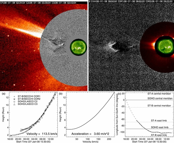
Figure 1. Remote observations of an ejecta or small-scale CME associated with the long-decay C1.4 X-ray flare of 2008 January 7, peaking around 15:30 UT, which occurred in AR 10980 located S10W03. Top: composite images on 2008 January 8, with the ejecta shown in difference images (left) around 2:30–2:42 UT with SOHO/EIT 195 Å and LASCO C2–C3, (right) around 8:50–9:22 UT with STEREO-B/SECCHI EUVI 195 Å, COR1, and COR2; the largest bright region in the 195 Å images indicates the location of AR 10980. Bottom: propagation direction analysis of the ejecta with (a) height-time profiles (symbols) from SOHO/LASCO, STEREO-B/COR1–COR2 and (thick line) after triangulation, giving a speed of 113.5 km s−1 from a linear fit; (b) velocity–height profile after triangulation giving an acceleration of 3.6 m s−2; (c) heliolongitude of the triangulated feature (thick line), with respect to the longitude of the Sun–Earth line, which shows an eastward deflection of the ejecta; a quadratic fit to the time series (dashed line) traces the origin of the ejecta close to the same longitude as AR 10980 at the time of the flaring; horizontal lines give the positions of central meridians and Eastern limbs as observed by each spacecraft, explaining in part how the ejecta becomes out of the fields of view of remote instruments.
Download figure:
Standard image High-resolution imageOne can first note a difference between the ejecta position angles as observed from SOHO and STEREO-B coronagraphs (upper panel of Figure 1). The measured heights of the ejecta in the plane of the sky can be seen as symbols in panel (a) of the lower plots in Figure 1. The SOHO/LASCO data points are from the CDAW CME catalog,8 which qualifies this event as "very poor" and indicates "central" and "measurement" position angles of 71° and 76°, respectively, indicating non-radial motion. The STEREO-B/COR imagery data points are obtained by way of elongation-time "J-maps" constructed at a fixed position angle of 83°–86°. By taking an average between the corresponding latitudes in the plane of the sky, the ejecta's heliolatitude can be estimated to be near 11°. In principle, one can easily determine the three-dimensional propagation direction of the ejecta by triangulation between the two sets of observations, overlapping in time. To proceed, second-order polynomial fits on each data set are interpolated to a regular time array and a simple triangulation method (Mierla et al. 2008) is applied with a separation angle of 22 9 between STEREO-B and SOHO. Panel (a) shows the resulting height of the ejecta (thick line), giving a speed of 113.5 km s−1 from a linear fit. The inferred velocity–height profile in panel (b) shows that the ejecta is slowly (3.6 m s−2) accelerated with speeds starting below 50 km s−1 up to 4 R☉ and reaching 240 km s−1 at a height of 13 R☉.
The heliolongitude of the triangulated feature (thick line in panel (c)) shows a strong eastward deflection of the ejecta until about 4UT on January 8, after which time the ejecta follows a track about 100° of heliolongitude east of the Sun–Earth line. A quadratic fit to the time series (dashed line) traces the origin of the ejecta close to the same longitude as AR NOAA 10980, located S10W03 from the Sun–Earth line, at the time when it produced a long-decay C1.4 GOES-class X-ray flare on 2008 January 7 (14:49–15:56 UT), peaking at 15:27 UT (the start time of the horizontal axis in panels (a) and (c) is 15:30 UT). Horizontal lines give the positions of central meridians and eastern limbs as observed by each spacecraft. This explains in part why the ejecta goes out of the fields of view of remote instruments from STEREO-A (propagating at angles behind the East limb as seen from STEREO-A). In addition, as noted above, the ejecta is rather faint. No trace of the ejecta could be found in difference movies from the Heliospheric Imager on STEREO-B. The ejecta may be too much inside the "Thomson sphere" for that spacecraft.
During this period of low solar activity, solar events are rare and rather isolated in time, so that there is a clear association in time between the ejecta detected by the coronagraphs and the X-ray flare detected on the disk. Although the association is partly confirmed spatially with both ejecta and flare events originating from the same heliolongitude as AR NOAA 10980, there is an apparent latitude difference between the events. To investigate this further, Figure 2 shows various Carrington maps, which derive from the photospheric field synoptic chart (panel (a)) at the time when the events took place (Rotation 2065), using a potential field source surface (PFSS) model with spherical source surface at 2.5 R☉ (Luhmann et al. 1999). The maps represent the global magnetic field configuration of the corona (panel (b)), variations with respect to the previous Carrington Rotation (panel (c)) as well as the associated radial flow at 5 R☉ (panel (d)). The latter map is from the "MHDweb" project of the Predictive Science Modeling Support for SECCHI and IMPACT (PREDSCI9). The dashed vertical line indicates the approximate Carrington longitude and time corresponding to the flare and transient release in the corona.
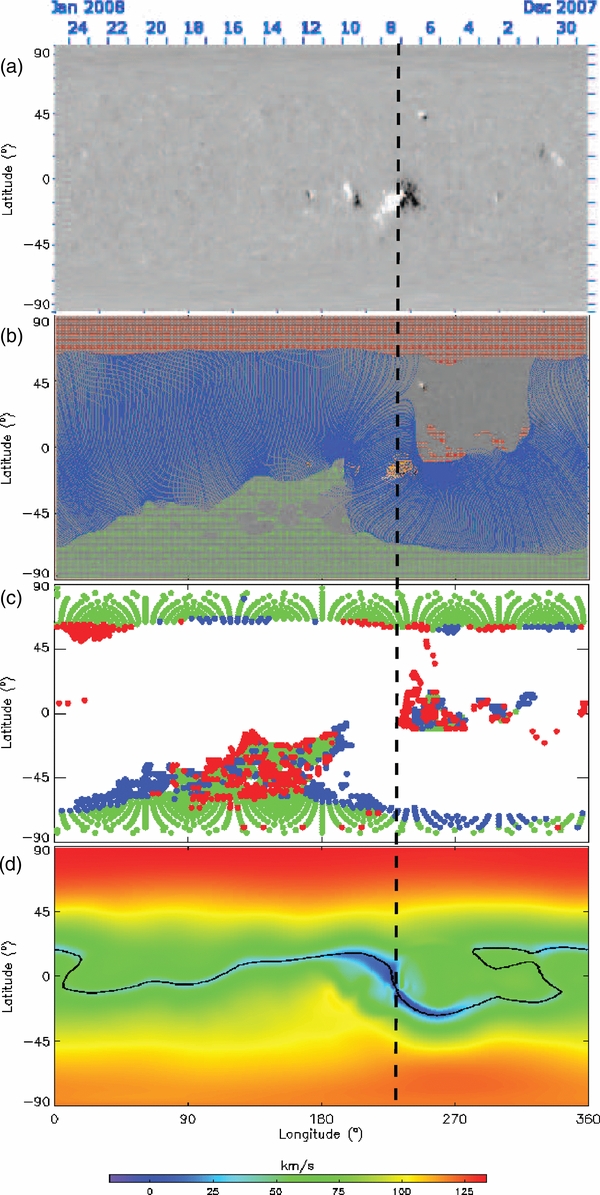
Figure 2. Carrington maps for Rotation 2065 showing (a) the photospheric magnetic field from the Global Oscillation Network Group, with increasing gray levels indicating negative (black) to positive (white) field values, (b) the PFSS model-derived global magnetic field configuration of the corona, showing open field regions (red and green), together with the projected field lines of the helmet streamer belt outer edge (blue), (c) variations with respect to Rotation 2064, showing those footpoints of field lines that differ by being newly closed (red) or opened (blue) as well as those in regions that remain open (green), and (d) radial flow at 5 R☉ together with the projected neutral line on the source surface from PREDSCI/MHDweb.
Download figure:
Standard image High-resolution imagePresumably at the origin of the combined solar event, the bipolar AR, centered on the disk, is located across the field inversion neutral line of the HCS, being thus at the base of the helmet streamer belt. Thus, the ejecta would appear to be directed equatorward, with a slight northward inclination. Although the ejecta is directed 100° east of the Sun–Earth line, it may already have considerable longitudinal extent while rising slowly. The strong longitudinal deflection under a slow motion is difficult to explain otherwise. The eastward direction of this deflection is an important feature, which will be addressed in Section 4. Very slow ejecta are reported to propagate outward in the plane of the sky with an initial low and constant speed ("velocity plateau"), before the ejecta is accelerated (e.g., Robbrecht et al. 2009; Shen et al. 2011, and references therein). This phase may correspond to swelling of the streamer (e.g., van der Holst et al. 2009). The magnetic field inversion line of the HCS is embedded in a streamer where the solar wind is below 50 km s−1 at 5 R☉ and moves to northern latitudes eastward of AR 10980 (panel (d)). This could explain the northward motion of the ejecta during its slow rise (below 4 R☉), with the maximum latitude excursion consistent with the average ejecta's heliolatitude of 11° and being reached about 45° longitude eastward to the source. Note that the difference in latitude between the eastern streamers seen on the plane of the sky from SOHO and STEREO-B is consistent with the latitude decrease of the inversion line with heliolongitudes further to the east (corresponding to the detection of a fainter streamer in COR1 as seen in Figure 1).
Of particular relevance for the connection with in situ phenomena is the presence of low-latitude coronal holes near the equator, on each side of the coronal streamer overlying AR 10980. These coronal holes have opposite sector polarities, with inward and outward interplanetary magnetic field (IMF) polarity connected to the northern and southern hemispheres, respectively (panel (b) of Figure 2). Panel (c) of Figure 2 indicates a large number of topological changes in both coronal holes, which could lead to much transient activity (Luhmann et al. 1998). In particular, the changes between Carrington Rotations are ordered in a way (closing westward, opening eastward of the streamer) suggesting differential rotation-driven evolution (Luhmann et al. 1999). The newly closing and opening coronal field lines are expected to form a boundary layer between the coronal holes and the helmet streamer belt (e.g., Lionello et al. 2005, 2006). Prior to the events reported here, flaring activity was low with AR 10980 being almost the only active source on the solar disk, producing occasionally GOES C-class, but mostly B-class flares. From this region, the previous flares were a C1.3 on January 2 (11:55 UT), a B1.8 on January 4 (03:19 UT), and a A8.4 on January 7 (05:52 UT). During this time period, 1–6 streamer puffs are detected per day with eastward trajectories and the timing is adequate to associate the above flares with one of them (see CDAW CME catalog). The X-ray levels remain below B-levels for the next 22 days (until a B1.2 flare on January 29 17:43 UT) and no more ejecta is detected until the next day. Being well positioned spatially, near the central meridian, and well isolated in time makes the C1.4 flare of January 7 (15:30 UT) a good solar event candidate for connection with in situ data.
3. IN SITU OBSERVATIONS
3.1. Overview of Multi-spacecraft Observations
We use the HCS and more generally the sector boundary as markers to relate solar and interplanetary phenomena and to inter-compare in situ observations at the different spacecraft. To identify the relevant sector boundary crossing, we select the one with a change from a toward to an away IMF sector polarity, occurring within a few days from the passage near the solar disk's central meridian of the magnetic field inversion line, inclined at equatorial latitudes near AR 10980. As illustrated in Figure 3, the associated HCS passage is detected by various spacecraft: at ∼15:30 UT, January 10 by STEREO-B, 23° east of the Sun–Earth line; at ∼12:30 UT, January 12 by the near-Earth spacecraft Advanced Composition Explorer (ACE), Wind and Cluster (in the solar wind); and finally at ∼21:30 UT, January 13 by STEREO-A, 213 west of the Sun–Earth line. The time lags between spacecraft are equivalent to longitudinal rotation periods of 30.3 days from STEREO-B to Earth and 23.6 days from Earth to STEREO-A. Those are consistent with the solar rotation period (∼27 days) and latitudinal corrections expected from the slightly higher and lower heliographic latitudes of STEREO-B and STEREO-A, respectively, from the Earth heliographic latitude (∼ − 4°), combined with the latitudinal profile of the magnetic field inversion line at the Sun (at a given heliographic longitude, the HCS crossing progresses in time from low to high latitudes; see Figure 2(d)).

Figure 3. Spacecraft positions, in the GSE Cartesian coordinate system, during the passage of the HCS on 2008 January 10–13 with normals at each spacecraft projected in (a) the noon-midnight meridional plane, (b) the ecliptic plane.
Download figure:
Standard image High-resolution imageThe sector boundary and its trailing edge are identified and described at each spacecraft with magnetic and plasma in situ observations, provided by the instruments listed in Table 1. Figures 4–6 give a three-day overview at each spacecraft (with ACE to represent the near-Earth spacecraft) including the sector boundary and the trailing region observed prior to the arrival of a corotating fast stream. Panels (a)–(d) show the magnetic field strength and Cartesian geocentric solar ecliptic (GSE) components. The polarity turns from toward (inward, Bx > 0) to away (outward, Bx < 0) IMF sector polarity. The electron pitch angle (P.A.) distribution in panels (e) indicates that the sector polarity transition contains a clear P.A. flip from 180° to 0°, allowing the detection of the true sector boundary (TSB). However, the sector boundary may correspond to periods without strahl, referred to as "heat flux dropout" (HFD). As shown below, the technique to identify the TSB may still be applied in the presence of residual strahls. Generally, the TSB is co-located with the major magnetic field reversal at the HCS. A common feature associated with the HCS is a reduction in the field magnitude, which is also one of the heliospheric plasma sheet (HPS) characteristics (Winterhalter et al. 1994). Panels (f)–(h) show respectively the proton density, Np, proton bulk flow speed Vp (|Vp|), and α-particle to proton density ratio, Na/Np. In all three passages, the HPS is indicated between vertical green lines and characterized by an increase in plasma density and decrease in magnetic field. In the away sector is shown the leading edge (blue vertical line) of a corotating fast stream (with Vp reaching speeds above 600 km s−1). The portion between the sector boundary and the fast stream contains a velocity enhancement reaching about 600 km s−1 at STEREO-B (near 22 UT on January 10) and at ACE (near 23 UT on January 12), but not seen at STEREO-A. We study and refer later to this stream as a CHBL stream.

Figure 4. Sector boundary of 2008 January 10, and its trailing edge observed by STEREO-B over a three-day interval. The plot shows (a) the total, (b)–(d) the GSE components of the magnetic field, (e) the color-coded P.A. velocity distributions f (v) of suprathermal electrons, in units of s3 km6, (f) the proton number density, (g) the proton bulk flow speed, and (h) alpha to proton density ratio. Vertical lines indicate the boundaries of the HPS (green) and the slow to fast speed stream interface (blue).
Download figure:
Standard image High-resolution image
Figure 5. Sector boundary of 2008 January 12, and its trailing edge observed by ACE over a three-day interval, with panels and vertical lines as in Figure 4.
Download figure:
Standard image High-resolution image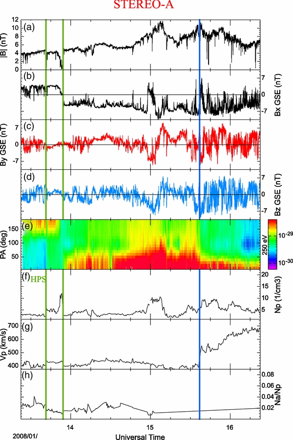
Figure 6. Sector boundary of 2008 January 13, and its trailing edge observed by STEREO-A over a three-day interval, with panels and vertical lines as in Figure 4.
Download figure:
Standard image High-resolution imageTable 1. Instruments Providing Magnetic Field and Plasma in situ Measurements in the Solar Wind
| Mission | Magnetic Field | Plasma |
|---|---|---|
| STEREO | In situ Measurements of Particles and CME Transients (IMPACT; Luhmann et al. 2008)–Magnetometer (MAG; Acuña et al. 2008) | IMPACT/Solar Wind Electron Analyzer (SWEA; Sauvaud et al. 2008), The Plasma and Suprathermal Ion Composition Investigation (PLASTIC; Galvin et al. 2008) |
| ACE | Magnetic Fields Experiment (MAG; Smith et al. 1998) | Solar Wind Electron Proton Alpha Monitor (SWEPAM; McComas et al. 1998), Solar Wind Ion Composition Spectrometer (SWICS; Gloeckler et al. 1998) |
| Wind | Magnetic Field Investigation (MFI; Lepping et al. 1995) | Solar Wind Experiment (SWE; Ogilvie et al. 1995) |
| Cluster | Flux Gate Magnetometer (FGM; Balogh et al. 2001) | Plasma Electron and Current Experiment (PEACE; Johnstone et al. 1997) |
Download table as: ASCIITypeset image
Figures 7–9 give an 8 hr overview of the HPS at each spacecraft. The three upper panels provide a close-up view of the magnetic field strength and normalized Cartesian GSE components (panels (a) and (b)) as well as the P.A. distributions (panels c). The latter are used to locate the TSB precisely, indicated with a blue vertical dashed line, by using residuals if necessary, in particular at STEREO-B, where the whole HPS corresponds to an HFD. This is used to show that the TSB and HCS are located on the trailing edge of the HPS. This location corresponds to a clear change between relatively stable (GSE) azimuthal magnetic field directions, as shown in panel (a) of Figure 10.
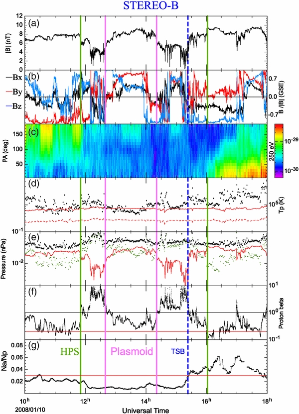
Figure 7. HPS of 2008 January 10, observed by STEREO-B over an 8 hr interval. The plot shows (a) the total, (b) the normalized GSE components of the magnetic field, (c) the color-coded P.A. velocity distributions f (v) of suprathermal electrons, in units of s3 cm6, (d) the proton temperature, (e) total (black), plasma (green) and magnetic (red) pressures, (f) the proton beta, and (g) alpha to proton density ratio. Vertical lines indicate the boundaries of the HPS (green, as in Figure 4), the boundaries of plasmoid(s) (purple), the TSB (blue dashed).
Download figure:
Standard image High-resolution image
Figure 8. HPS of 2008 January 12, observed by ACE over an 8 hr interval, with panels and vertical lines as in Figure 7.
Download figure:
Standard image High-resolution image
Figure 9. HPS of 2008 January 13, observed by STEREO-A over an 8 hr interval, with panels and vertical lines as in Figure 7.
Download figure:
Standard image High-resolution image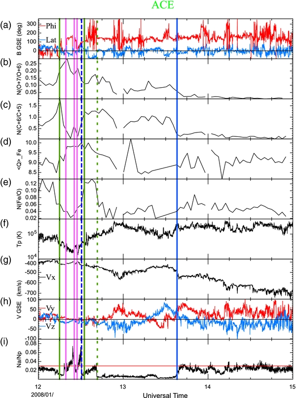
Figure 10. Sector boundary of 2008 January 12, and its trailing edge observed by ACE over a three-day interval. The plot shows (a) the elevation and azimuthal (mod π) components of the magnetic field, (b) the oxygen abundance ratio N(O7 +/O6 +), (c) the carbon abundance ratio N(C6 +/C5 +), (d) the iron charge state 〈Q〉Fe, (e) the iron to oxygen abundance ratio N(Fe/O), (f) the proton temperature, (g)–(h) Cartesian GSE components of proton velocity, and (i) the alpha to proton density ratio. A dashed green vertical line indicates the transition between two portions of CHBL of different origins (streamer leg on the HPS side and streamer cusp on the fast stream side). Other vertical lines are as in Figures 5 and 8.
Download figure:
Standard image High-resolution image3.2. Plasma Structures in the HPS as Plasmoids
3.2.1. Main Proxies
We now take a closer look at plasma structures, in the HPS, which are indicated between purple vertical lines in Figures 7–9. Although they appear different between the spacecraft, several proxies indicate that these structures are consistent with near-pressure-balanced plasmoids, corresponding to a certain class of small-scale ejecta or ICME. Small-scale transients in the slow solar wind have been identified with far fewer signatures than those found in classical ICMEs (Kilpua et al. 2009). The additional difficulty here is to identify these structures embedded in the HPS, which is a high-beta plasma environment, similar to the magnetotail plasma sheet. In this context, we combine two approaches, that used for identification of transients in the solar wind and that used for plasmoids in the magnetotail.
First, a large part of the intervals proposed show all depressions in (radial) proton temperature Tp (black line in panels (d)) as compared to adjacent regions. Low Tp, relative to the expected temperature, Tex, for normally expanding solar wind, is considered a very robust signature of transients (Lopez 1987). Tex (plain red line) is the typical temperature found in the solar wind and is inferred using an empirical correlation between the proton temperature and Vp (shown in Figures 4–6), which is here specific to the ACE/Solar Wind Electron Proton Alpha Monitor instrument (Neugebauer et al. 2003). The first plasmoid at ACE with Tp < Tex/2 (dashed red line) is fully consistent with the signature of ICME passage (Richardson & Cane 1995). Although they would require empirical determination of the temperature threshold at both STEREO spacecraft, a large part of the intervals proposed for the other plasmoids at STEREO-B, ACE, and STEREO-A corresponds to a region where Tp ⩽ Tex and, in any case, where Tp is lower than its surroundings.
Second, plasmoids can usually be identified in the magnetotail plasma sheet by total pressure enhancements (TPEs) with respect to the background (Ieda et al. 1998). If the TPE is due to plasma (or inversely magnetic) pressure enhancement, then the plasmoid is categorized to be of magnetic − island (or inversely flux − rope) type. Panels (e) show total (black), plasma (green), and magnetic (red) pressures. High-resolution electron temperatures from Wind and Cluster (not shown) indicate values of ∼105 K, much greater than the proton temperatures. While electron thermal pressures are not included in the magnetotail, their inclusion appears crucial in the solar wind to give a proper treatment of the identification of plasmoids. We thus assume an electron–proton plasma and count the plasma pressure as double of the proton pressure at the STEREO and ACE spacecraft. In general, the structures are near pressure-balanced, i.e., the total pressure in the plasmoids does not differ markedly from the total pressures in the surrounding plasma of the HPS. Plasma and magnetic pressure variations are most apparent at STEREO-B and A and allow the detection of plasmoids based on these variations. A flux-rope-type plasmoid is generally found at each spacecraft: in the middle of the HPS, at STEREO-B and A, or marginally on the trailing edge of the HPS, for the proposed second plasmoid at ACE. The first plasmoid at ACE, in the middle of the HPS, has higher plasma than magnetic pressure and therefore can be classified as of magnetic-island type. Using exact pressures from the measurements at Wind, the total pressures in plasmoids 1 and 2 are 0.02 ± 0.001 and 0.035 ± 0.006 nPa, respectively, and magnetic pressure contributions are 12(± 8)% and 48(± 37)%, respectively, consistent with Plasmoid 2 being marginally of flux rope type.
Third, as shown in panels (f), the flux-rope-type plasmoids have low proton plasma beta, βp (mostly below 0.5), relative to the higher-βp HPS environment. Although the detected plasma structures in the HPS do not conclusively qualify as magnetic-cloud-like structures according to criteria in the ambient solar wind (an acceptable proxy for such structures would be values of βp ⩽ 0.2; e.g., Foullon et al. 2007), there are no previous report on the relevant thresholds inside the high-βp HPS. The magnetic field values, in the range of 2–8 nT, are consistent with values found in slow solar wind transients and, more precisely, are intermediate between the lowest values of 2 ± 1 nT associated with large-scale field reversals close to the HCS (Foullon et al. 2009, 2010b) and the 7.3 ± 1 nT average value of magnetic field maximum reported in other small-scale structures, that are somewhat larger and detected farther away from the HCS (Kilpua et al. 2009). In fact, low levels of magnetic fluctuations are observed, for instance in the magnetic field components (panels (b)), even in the magnetic-island case at ACE. The regular, smooth, and low variance magnetic field, which may or may not have a coherent rotation, is indicative of a flux-rope-type magnetic structure and is generally accompanied by a magnetic pressure larger than the plasma pressure, corresponding to the flux rope type of plasmoid.
3.2.2. Other Properties
We examine in more detail the geometry of the plasmoids. We first compute the normal directions to individual plasmoid boundaries and the HCS, forming magnetic discontinuities in the HPS. We either perform single-spacecraft techniques across the boundary portions of magnetic field time series at each spacecraft or a four-spacecraft timing analysis on magnetic field data at Cluster. The single-spacecraft techniques include (1) a minimum variance analysis (MVA), (2) the constrained MVA with null magnetic field normal component (MVABN), (3) the cross-product between magnetic field vectors measured before and after the given time interval, and (4) an MVA using an alternative variance matrix (MVAS; Siscoe et al. 1968). The MVA results are acceptable when a well-defined set of eigenvectors, denoted  ,
,  , and
, and  (corresponding respectively to minimum, intermediate, and maximum variance directions) is returned. We consider this condition fulfilled when the intermediate to minimum eigenvalue ratio, λj/λi, is larger than 10 (e.g., Sonnerup & Scheible 1998; Knetter et al. 2004). If the MVA results are not acceptable, we consider the MVABN results to be justified when the average of the minimum to total field magnitude ratio, 〈Bi/B〉, (from MVA) is less than 0.1. We then consider the magnetic coplanarity normals obtained via cross-product analysis to be valid if they agree with at least one of the MVA or MVABN results (to agree, the difference angle must be less than 15°). In the last resort, we consider the MVAS results to be acceptable when λj/λi > 10. The results that satisfy the above criteria or agree with the reliable ones are indicated with an asterisk in Table 2. Trusted normal directions are computed using the average of the validated results. As well as the surface normal vector
  , four-spacecraft timing provides estimates of the velocity VN, along the discontinuity normal directions (Russell et al. 1983). This method assumes a discontinuity to be close to planar and to move with constant velocity on the scale size of the spacecraft separation. The four Cluster spacecraft are arranged at this time in a triangle configuration, with C3 and C4 relatively close (50 km apart) and C1, C2, and C3 roughly 8800 (±1720) km apart.
Table 2. Results of Single-spacecraft MVA, Cross-product Analysis, and four-spacecraft Timing Analysis for the Magnetic Discontinuities in the Sector Boundary of 2008 January 10–13
| S/C | Dis. | Time (UT) | Analysis |  (GSE) (GSE) |
Notes | VN/Nx |
|---|---|---|---|---|---|---|
| (km s−1) | ||||||
| ST-B | 2008 Jan 10 | |||||
| Plasmoid | 12:39:30–14:21:01 | MVA | [−0.910, 0.415, 0.003] | λj/λi = 12.5 | ||
| HCS | 15:11:27–15:34:16 | MVA | [−0.849, −0.341, 0.403] | λj/λi = 14.8 | ||
| Near Earth | 2008 Jan 12 | |||||
| ACE | P1a | 07:58:42–08:04:03 | MVA | [−0.189, 0.942, 0.278] | λj/λi =5.2 | |
| MVABN | [−0.649, −0.348, 0.676]* | 〈Bi/B〉 = 0.09 | ||||
| Crossed-B | [−0.576, −0.421, 0.701]* | |||||
| T. average | [−0.613, −0.385, 0.690] | |||||
| P1b | 10:07:02–10:10:51 | MVA | [−0.297, 0.364, 0.883] | λj/λi = 17.7 | ||
| P2a | 10:54:33–10:57:32 | MVA | [−0.560, −0.815, 0.148 ] | λj/λi = 8.9 | ||
| MVABN | [−0.227, −0.061, −0.972]* | 〈Bi/B〉 = 0.94 | ||||
| Crossed-B | [−0.267, 0.051, −0.962] | |||||
| MVAS | [−0.227, −0.061, −0.972]* | λj/λi = 96.2 | ||||
| T. average | [−0.227, −0.061, −0.972] | |||||
| HCS | 12:09:49–12:12:40 | MVA | [−0.906, −0.230, 0.355] | λj/λi = 17.3 | ||
| P2b | 12:52:37–13:00:15 | MVA | [−0.913, −0.362, −0.188] | λj/λi = 19.8 | ||
| Wind | P1a | 08:17:30–08:21:45 | MVA | [−0.636, −0.764, −0.109]* | λj/λi = 0.8 | |
| MVABN | [−0.661, −0.750, −0.014]* | 〈Bi/B〉 = 0.09 | ||||
| Crossed-B | [−0.628, −0.772, −0.097]* | |||||
| T. average | [−0.642, −0.763, −0.073] | |||||
| P1b | 09:56:04–09:57:20 | MVA | [−0.380, −0.393, −0.837] | λj/λi = 3.5 | ||
| MVABN | [−0.265, 0.420, −0.868]* | 〈Bi/B〉 = 0.29 | ||||
| Crossed-B | [−0.211, −0.904, 0.373] | |||||
| MVAS | [−0.279, 0.370, −0.886]* | λj/λi = 10.5 | ||||
| T. average | [−0.272, 0.395, −0.877] | |||||
| P2a | 10:52:57–10:53:31 | MVA | [−0.729, −0.178, −0.661] | λj/λi = 11.0 | ||
| HCS | 12:15:09–12:19:56 | MVA | [−0.706, −0.620, 0.341]* | λj/λi = 9.0 | ||
| MVABN | [−0.692, −0.639, 0.337]* | 〈Bi/B〉 = 0.01 | ||||
| Crossed-B | [−0.771, −0.540, 0.338]* | |||||
| T. average | [−0.724, −0.601, 0.339] | |||||
| P2b | 12:51:56–12:58:46 | MVA | [−0.834, −0.480, −0.272] | λj/λi = 13.7 | ||
| Cluster | P1a | 08:44:06 +[9.1, −16.3, 11.1, 11.4] | 4-sc | [−0.759, −0.637, −0.137] | VN = 225.1 km s−1 | −296.6 |
| P1b | 10:41:11 +[11.9, 18.4, −19.4, −19.4] | 4-sc | [−0.660, −0.308, 0.685] | VN = 118.0 km s−1 | −178.8 | |
| P2a | 11:30:35 +[−3.9, 48.2, −55.3, −55.8] | 4-sc | [−0.255, −0.162, 0.953] | VN = 73.3 km s−1 | −287.5 | |
| HCS | 12:59:21–12:59:25 | C2 MVA | [−0.980, −0.037, 0.196] | λj/λi = 15.2 | ||
| 12:59:30 +[4.3, −6.8, −5.2, −5.1] | 4-sc on Bk | [−0.965, −0.221, 0.141] | VN = 280.6 km s−1 | −290.8 | ||
| P2b | 12:14:40 +[6.2, 5.6, −5.9, −5.8] | 4-sc | [−0.640, −0.497, 0.587] | VN = 166.0 km s−1 | −259.4 | |
| ST-A | 2008 Jan 13 | |||||
| HCS | 21:29:06–21:49:11 | MVA | [−0.246, −0.775, 0.582]* | λj/λi = 5.8 | ||
| MVABN | [−0.133, −0.701, 0.700]* | 〈Bi/B〉 = 0.1 | ||||
| Crossed-B | [−0.218, −0.719, 0.660]* | |||||
| T. average | [−0.200, −0.734, 0.650] | |||||
Notes. The table lists, from left to right, the spacecraft concerned, the discontinuity name, the time interval or crossing time (at C1, C2, C3, and C4), the analysis technique, the obtained normal vector  in GSE Cartesian coordinates, and notes. The techniques are either the MVA, MVABN, cross-product, MVAS or trusted average from the preceding results (indicated with an asterisk), as well as four-spacecraft timing. The final result retained is highlighted in bold. The notes may include the eigenvalue ratio, λj/λi, the average ratio of the normal component to the total magnetic field, 〈Bi/B〉, and the velocity VN along the discontinuity normal obtained from four-spacecraft timing, for which the radial speeds VN/Nx are added in the last column.
Download table as: ASCIITypeset image
The resulting directions are highlighted in bold in Table 2 and projected on different GSE planes in Figures 3 and 11, pointing in the downstream direction by convention. In Figure 3, the normals to the HCS at the different spacecraft show that the HCS curves along the Parker spiral. MVA through the plasmoids returns reliable results (λj/λi > 10) only for the flux-rope plasmoid at STEREO-B. The minimum variance direction is given in Table 2 and indicates a flux-rope axis orientation lying in the ecliptic plane and pointing 39° overall westward from the plane of the HCS. In Figure 11, we examine differences between spacecraft for the plasmoids detected near Earth. The spacecraft positions are shifted sunward along the Sun–Earth line, with respect to the positions at the passage time of the first recorded discontinuity, P1a (at ACE), based on an average solar wind speed of VSW = 433 km s−1 and the time duration between the discontinuity arrivals. In this reference frame, there is a good correspondence between HCS discontinuities in their alignment across the Sun–Earth line and in their orientation. The discontinuities adjacent to the HCS do not align so well across the Sun–Earth line. In addition, the velocities at Cluster projected along the Sun–Earth line (VN/Nx in Table 2) indicate larger radial speeds at the leading edges of plasmoids, P1a and P2a, compared to the trailing edges, P1b and P2b. The different propagation times can explain the reported misalignment, with transients expanding in their leading part and being slightly slower in their trailing part. As shown in Foullon et al. (2009) using Cluster, the slow solar wind transients are broadly convected with the solar wind, but occasional non-planar structures (as small as the Cluster spatial scale) and associated outflows or Alfvénic fluctuations can be present (which may affect the timing analysis). Here the bulk flow speed inside the plasmoids at ∼420 km s−1 is 20–30 km s−1 lower than in the ambient HPS. Such differences in bulk flow speeds were also occasionally found within small-scale transients (Kilpua et al. 2009). Overall, the plasmoids have sizes of about 500 ± 100 RE = 3, 200, 000 ± 640, 000 km, intermediate between the transient sizes studied by Foullon et al. (2009, 2010b) and that by Kilpua et al. (2009).

Figure 11. Normals to the discontinuities P1a, P1b, P2a, P2b, and the HCS, on 2008 January 12, projected in (a) the noon-midnight meridional plane and (b) the ecliptic plane. The spacecraft positions of ACE, Wind and Cluster are shown as full circles. The discontinuity normals are shown at spacecraft positions shifted sunward along the Sun–Earth line, with respect to the positions at the passage time of the first discontinuity, P1a (at ACE).
Download figure:
Standard image High-resolution imageTo interpret the magnetic topology of field lines, we use electron P.A. characteristics presented in panels (c) of Figures 7–9. This method can be complicated by the extent of HFD occurring in the vicinity of the HCS (Foullon et al. 2010b). At STEREO-B in particular, the whole HPS corresponds to an HFD and appears as a double density structure embedding the flux-rope-type plasmoid (indicated by a higher magnetic pressure). The occlusion of an ICME "in the HCS" was previously inferred by Crooker & Intriligator (1996), but there were no electron P.A. distributions in that work. A counterstreaming signature of suprathermal electrons would be generally expected to signal nested magnetic loops overlying the flux rope and being still connected to the Sun (Gosling et al. 1987). For this reason, to our knowledge, the plasmoid structure within an HFD at the HCS is the first one reported of its kind. The information about the connectivity to the Sun might be lost due to full or partial disconnection. At ACE, we identify possible traces in the residual strahls of counterstreaming and unidirectional electrons in the magnetic-island-type- and flux-rope-type plasmoids. At STEREO-A, we have unidirectional electrons typical of the toward sector in the flux-rope-type plasmoid. Thus, the P.A. distribution at ACE appears intermediate between those of STEREO-B and STEREO-A.
Finally, Na/Np is highly variable inside a given ejecta and may differ markedly from the typical ratio observed in the solar wind, reaching lower values and also values as high as ∼20% (Borrini et al. 1982; Galvin et al. 1987). The typical ratio was found to rise from less than 2% near solar minimum to about 5% near solar maximum and to vary with solar wind speed (Aellig et al. 2001). In particular, during the previous solar minimum, for Vp in the range 400–450 km s−1, the typical ratio was found around values of 3%. Panels (g) of Figures 7–9 show that the ratio obtained with ACE and STEREO reaches a minimum of ∼1% and a maximum of ∼7% (at ACE) in the interval proposed for the ejecta, confidently lower or higher than the typical 3% average value (indicated by a horizontal red line). The α-particles may be good indicators of flare plasma (see also Foullon et al. 2007). At ACE, the ratio has a double-peaked structure associated with the two plasmoids. According to Suess et al. (2009; see their Figure 11), their plasma origin corresponds to the legs of streamers.
To summarize, although the detected plasma structures in the HPS do not, in principle, qualify as magnetic-cloud-like structures (the plasma beta is not low enough as one would expect for classical ICMEs in the ambient solar wind), we propose that they can still qualify as structures of the sort since they are low-βp structures relative to the higher-βp HPS environment (one of them can be treated with MVA). Although they would require empirical determination of the temperature threshold at both STEREO spacecraft, the structures all have depressions in Tp and thus, together with the 20–30 km s−1 lower bulk flow speed at ∼420 km s−1, can qualify as slow ICMEs. They can most probably be qualified as plasmoids, although they remain near pressure-balanced (they have no substantial TPEs). None of the structures seem to have bidirectional electrons, except perhaps in the residual strahls at ACE. We note that the HPS plasmoids have length scales on average 13 times smaller than the typical radial cross-sections of 0.249 ± 0.078 AU for magnetic clouds obtained at average speeds of 455 km s−1 (Lepping et al. 2006). Their magnetic field values (5 ± 3 nT) are more than three times smaller than the typical 17.1 ± 5.9 nT found for the same magnetic cloud data set. A final difference to note is that the one resolved flux-rope axis orientation at STEREO-B lies in the ecliptic plane but not close to the Y-axis, contrary to magnetic clouds.
3.3. CHBL Properties
In this section, we refer principally to Figure 10, which shows additional properties observed at ACE, in time series spanning the same three-day interval as used in Figure 5. Panels (b)–(e), in particular, show ion composition signatures from the Solar Wind Ion Composition Spectrometer: first (b) the oxygen abundance (density) ratio between O7 + and O6 +, N(O7 +/O6 +), next (c) the C6 + and C5 + abundance ratio, N(C6 +/C5 +), then (d) the average iron charge state composition, 〈Q〉Fe, and finally (e) the Fe and O abundance ratio, N(Fe/O).
We use auxiliary Figures 12 and 13 to differentiate some of those properties between the separate regions identified within the three-day interval. N(O7 +/O6 +) and N(C6 +/C5 +) are plotted versus the proton bulk flow speed, Vp, in panels (a) and (b) of Figure 12, respectively. N(O7 +/O6 +) can be directly inverted into the "freeze-in" temperature of oxygen, TO76. Similarly, N(C6 +/C5 +) corresponds to a coronal source temperature, TC65 (e.g., Geiss et al. 1995; Hefti et al. 2000; McComas et al. 2002). The stream feature (interval with a velocity enhancement, between the HPS and the "slow to fast" speed stream interface) is represented with blue ×-crosses and is clearly seen to correspond to a CHBL, with a solar wind speed increasing monotonically with gradually changing abundances that correspond to decreasing freeze-in temperatures. In the CHBL stream, TO76 or TC65 range between 1.1 and 1.4 MK, intermediate between the fast stream and HPS freeze-in temperatures.
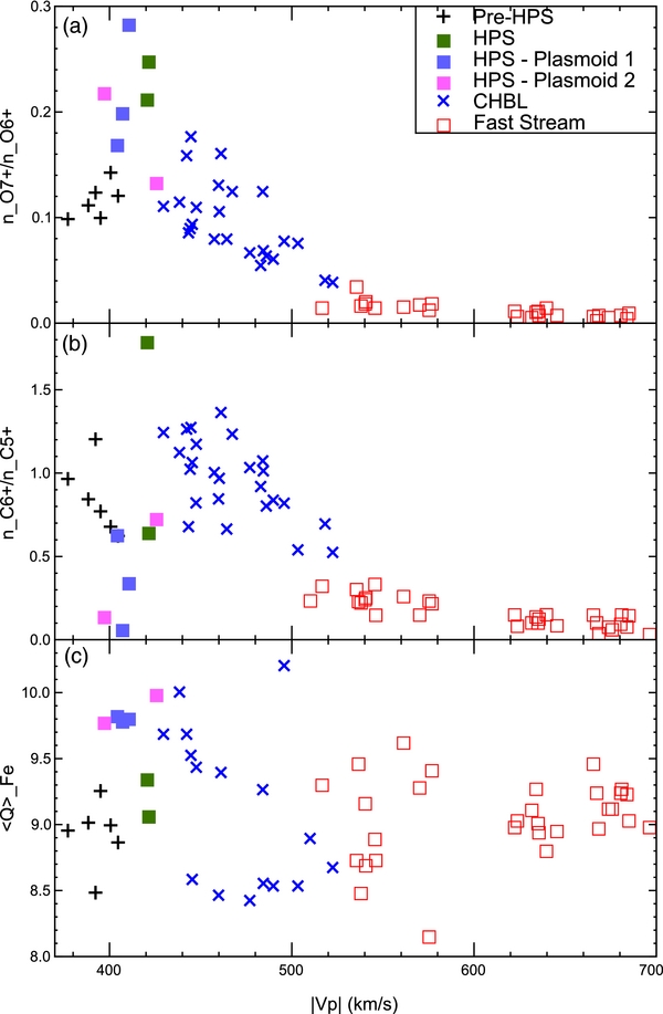
Figure 12. Ion composition characteristics, earmarked between the different regions of interest, vs. proton solar wind speed at ACE over the three-day interval shown in Figure 10. The plot shows (a) the oxygen abundance ratio N(O7 +/O6 +), (b) the carbon abundance ratio N(C6 +/C5 +), and (c) the iron charge state 〈Q〉Fe.
Download figure:
Standard image High-resolution image
Figure 13. Iron charge state, earmarked between the different regions of interest, vs. proton solar wind speed at STEREO-B, ACE, and STEREO-A, over the three-day intervals shown in Figures 4–7.
Download figure:
Standard image High-resolution image〈Q〉Fe is also plotted versus Vp and earmarked between the different regions of interest in Figure 12(c). This plot is reproduced in the middle panel of Figure 13 for comparison with counterparts at STEREO-B and STEREO-A (in the upper and lower panels, respectively). Interestingly, 〈Q〉Fe does not differ between all the plasmoids observed at STEREO-B, ACE, and STEREO-A, at the highest values around 〈Q〉Fe ∼ 9.5–10. Such enhancements of 〈Q〉Fe have also been reported by Simunac et al. (2010) and K. Simunac et al. (2011, in preparation) in the HPS. Our study indicates that the major enhancement comes from the plasmoids within the HPS. A spread in 〈Q〉Fe within the CHBL is also observed at all spacecraft, including the non-stream region at STEREO-A. The values are somewhat lower in the fast stream, but only at STEREO-A can one see a clear drop in 〈Q〉Fe at the slow to fast stream interface, as reported and discussed by Galvin et al. (2009, and references therein). Overall, the CHBL appears to have iron charge states intermediate between the HPS and fast stream, but with a variable degree of differentiation.
As shown in Figure 10(e), the Fe/O ratio at ACE decreases by half at the leading edge of the CHBL from about 0.13 at 15:07 UT to about 0.05 at 17:07 UT on January 12. There is no gradual Fe/O ratio profile in the remaining larger portion of the CHBL, contrary to the freezing-in temperature profiles above. This difference between ion composition and freezing-in temperature profiles indicates that most of the CHBL source lays within the edge of the coronal hole, consistent with the statistical results of McComas et al. (2002). We explore the associated plasma properties in the following panels (f)–(i) of Figure 10, showing (f) temperature Tp, (g–h) Cartesian GSE components of proton velocity, and (i) Na/Np. One interesting fact is that Tp is clearly enhanced in the larger CHBL portion and more like the high-speed stream that follows. Moreover, deviations in the GSE components, Vy and Vz, of the flow perpendicular to the Sun–Earth line are observed in this CHBL portion, with relative speeds reaching about 50 km s−1 in both directions. First, as it reaches its maximum radial speed, the plasma of the CHBL is pushed toward the west and south, as in the high-speed stream. As its speed diminishes toward the "slow to fast" stream interface, the CHBL flow then reverses toward the east and north, before being restored to the fast stream directions. The latter opposite flows are considered to be the consequence of magnetic pressure build-up ahead of the fast stream catching up the slower wind. Together with temperature and solar wind speed local increases (panels (f)–(g)), density and magnetic field intensity local increases followed by decreases (Figures 5(a) and (d)), the latter flow deviations indicate the formation of forward and reverse shocks (Belcher & Davis 1971). We conclude that the largest portion of the CHBL at ACE is of fast stream origin.
By contrast, the portion of CHBL directly adjacent to the HPS, between 13 UT and 16:30 UT, is initially of streamer origin (chromospheric source, as indicated by the high Fe/O ratio). This portion of the CHBL is not depleted in helium (Figure 10(i)), which points to a streamer-leg origin. Furthermore, the transition between the two CHBL portions (indicated by a green vertical dotted line) is consistent with the trailing edge of a sector boundary layer, where the HCS is more or less centered and the elevation angle, which completes the magnetic field vector in panel (a) of Figure 10, approaches zero near its edge (Klein & Burlaga 1980; Foullon et al. 2009).
Although we currently lack calibrated data on the freeze-in abundance ratios at STEREO-A and STEREO-B, the CHBL identified at ACE can be inferred at STEREO-B based on the similarity of its fast speed stream and can also be related to the slower feature identified at STEREO-A. The average speed in the CHBL streams decreases from 509 km s−1 at STEREO-B to 478 km s−1 at ACE and 413 km s−1 at STEREO-A. In the directions of the HCS normal orientations, the corresponding thickness of the CHBL streams represents approximatively 52, 43, and 15 × 106 km, respectively. The largest portion of the CHBL stream at ACE is depleted in helium and, most puzzlingly, no helium depletion is observed in the corresponding stream at STEREO-B or interval at STEREO-A (Figures 4–6(f)). Thus, the He-depleted CHBL stream at ACE, which would appear to be both of fast stream and streamer cusp origin, is outstanding.
4. DISCUSSION
4.1. Plasmoid Releases and the HPS Formation
Figure 14 summarizes the observations and is helpful in interpreting the in situ signatures in the solar wind. In Section 3.2, we established the presence of various sections of (near-pressure-balanced) flux-rope- and magnetic-island-type plasmoids within the HPS, associated with the HCS corotating past STEREO-B, near-Earth spacecraft ACE, Wind and Cluster, and STEREO-A. In Section 2, we showed that the ejecta locus of interest within or along the HCS is located 100° east of the Sun–Earth line at 15:30 UT on 2008 January 8. The initial ejecta speed of 240 km s−1 at 13 R☉ is much too slow to expect it to reach 1 AU two days later. In any case, the crossing of the HCS two days later by STEREO-B is likely to correspond to equatorward positions, westward of this locus, in fact close to the flaring AR 10980's position. It is possible that the ICME forms a highly distended occlusion in the HCS (Crooker & Intriligator 1996) and that the ejecta's western edge can propagate along the HCS surface at positions connected to the associated flaring longitude. However, even in this case, for it to be detected in situ at STEREO-B as an occlusion in the HCS, it would have to reach average transit speeds much larger than the in situ bulk flow speeds within the HPS. Thus we rule out the flux-rope-type plasmoid at STEREO-B to be the direct counterpart of the slow ejecta observed remotely on 2008 January 7. There still remains the possibility that the plasmoid at STEREO-B is the counterpart of an earlier slow streamer puff. In particular, one likely candidate is detected on 2008 January 4, following a B1.8 GOES-class flare peaking at 03:12 UT and attributed to AR 10980, with similar properties to the January 7 event studied in Section 2 ("very poor event" in SOHO/LASCO catalog, with first C2 appearance at 07:54 UT and with central position angle of 93°).
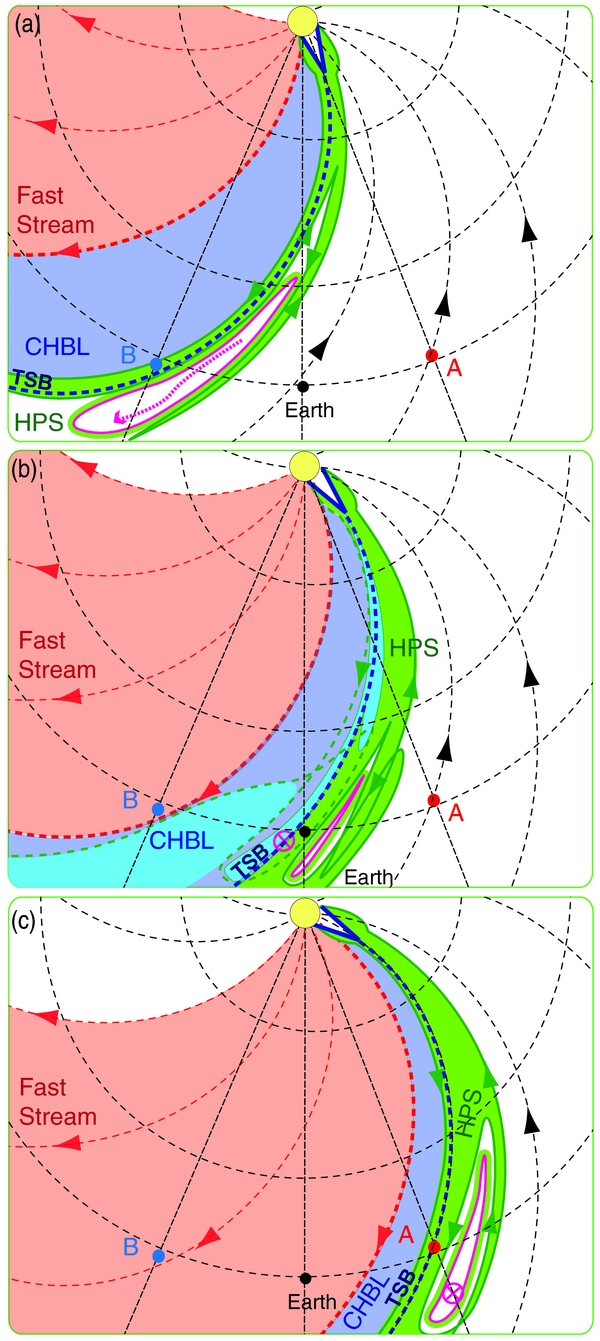
Figure 14. Patterns of outflowing loops embedded in the sector structure and properties of CHBL, determined from the observations at (a) STEREO-B, (b) near Earth, and (c) STEREO-A. The toward and away sectors are shown with black and red arrows, respectively, in the ecliptic plane and are separated by the HCS coinciding with the TSB (dark blue dashed line). STEREO-B, Earth, and STEREO-A are indicated by circles filled in blue, black, and red, respectively. The green, blue, and red areas represent the HPS, CHBL, and fast stream, respectively. Regions depleted in helium are shown in light blue in panel (b). Plasmoids are indicated in purple contours and/or arrows for flux-rope types. In panel (a), the curved dashed purple arrow represents the projected main axis of the flux-rope plasmoid observed at STEREO-B. In panels (b) and (c), the unresolved axis of flux-rope-type plasmoids is represented with arrows pointing into the ecliptic plane.
Download figure:
Standard image High-resolution image
The association found here between a flux-rope-type plasmoid and an HFD indicates that an HFD, usually associated with disconnection in the solar wind (or interchange reconnection and scattering), could also be connected with the formation and motion of a "quiescent" plasmoid in the fully or partially disconnected bundle of flux. Furthermore, the HPS plasma is much more dense at STEREO-B than at the other spacecraft. While this could have indicated a type of slow wind stream from long-decay X-ray event (Švestka & Fárník 2005), there are no He-rich flare plasma signatures. In fact, the denser plasma forms a double structure, which surrounds the plasmoid. Thus, this is interpreted instead as the boundary layer or sheath resulting from the interaction between the plasmoid and the ambient plasma required to produce the near speed-equalized and pressure-balanced HPS. Magnetic discontinuities, as observed in these surrounding structures, may correspond to Alfvénic fluctuations expected to develop in the compressed layer, which can lead to magnitude decreases (Tsurutani et al. 2007), where the magnetic field is lower than in both the plasmoid and the ambient plasma. Based on similarities in oxygen ion composition between phenomena, Liu et al. (2010) concluded that the proton density enhancements detected in situ in the vicinity of the HCS were likely to be caused by blobs originating from the streamer belt. Our study specifies that the association is due to the sheath of those blobs. It also offers a possible interpretation for the case of an HFD associated with a density increase ahead of a CIR in an event presented by Rouillard et al. (2010b) and for which no clear association with remote observations could be found. We find it consistent with the plasma layer being later compressed in the solar wind.
After five days following the ejecta's coronal release at 13 R☉, with average transit speed of 350 km s−1, intermediate between the remote and in situ speeds, the ejecta's detection at 1 AU and at ACE is more likely. The ACE plasmoids are not "quiescent" since they are related to He-rich solar flare plasma. The flux-rope-type (second) plasmoid at ACE is therefore a good candidate for the in situ counterpart of the twisted small-scale streamer ejecta observed remotely. After more than six days, the in situ observations at STEREO-A are likely to correspond to a new plasmoid. According to Crooker et al. (2004b), field reversals adjacent to the HCS can be interpreted as a pattern of loops magnetically opened by interchange reconnection. The electron P.A. distributions at ACE and STEREO-A imply some interchange reconnection configurations, with the magnetic-island-type (first) plasmoid at ACE and the flux-rope plasmoid at STEREO-A contained within the interchanged loop in the toward sector (see Figures 14(b) and (c)). The plasmoid signatures are also accompanied by the same type of surrounding compressed layers as inferred at STEREO-B, characterized by more scattering or HFD (panels (c) of Figures 8–9). The plasmoid at STEREO-A could be the counterpart of a later slow streamer puff, following the event studied in Section 2. One likely candidate is detected on 2008 January 8, possibly associated with micro-flaring activity between 15:30 and 19 UT (RHESSI flare list10) and a slow ejecta directed eastward ("very poor event" in SOHO/LASCO catalog, with first C2 appearance at 22:06 UT and with central position angle of 128°). In any case, the in situ observations are consistent with the idea that the release of plasmoids is continuous within the HPS. Thus, we conclude that what could maintain the high density in the HPS is the sheath of those plasmoids. Moreover, in the HPS, the decreasing values of proton density (presumably related to the plasmoid sheaths being less compressed) and the decreasing extent of the HFD or increasing strahl content (presumably related to the magnetic topology of plasmoids becoming more connected to the Sun) are interpreted as evolving properties from pre- to post-event cross-sections in the current sheet.
4.2. Plasmoid–CHBL Interaction and the CHBL Evolution
There is much to learn from making the connection between the flux-rope plasmoid at ACE, located across the TSB, and the slow ejecta, observed remotely to be accelerated. The acceleration of a slow ejecta is rarely reported in three dimensions (see also Bisi et al. 2010 for another event studied with other instruments). Thanks to two vantage points with SOHO/LASCO and STEREO-B/SECCHI, we have obtained a strong longitudinal deflection under a slow motion in Section 2, which we ascribed to the small-scale streamer ejecta reaching considerable longitudinal extent, while rising slowly in a swelling streamer. The eastward direction of the longitudinal deflection indicates a likely interaction with the coronal hole in the away sector. The two sides of the plasmoid across the TSB are clearly different, e.g., with He enrichment in the toward sector and depletion in the away sector. This two-sided plasmoid is likely to correspond to the type of blob envisaged by Suess et al. (2009; their Figure 15), which experiences a flow shear. This type of blob is shown in Figure 14(b), where the regions depleted in helium of cusp origin are shown in light blue. Note that the first (island-type) plasmoid at ACE in the toward sector is somewhat also two sided with a similar He enrichment on the slower side of the field reversal. However, the faster side is not as He-depleted as for the plasmoid located at the TSB. In Section 3.3, we established the presence of a CHBL adjacent to the HPS, with an outstanding He depletion in the largest portion ahead of the fast stream; we also showed that the chromospheric source of the smaller portion of the CHBL, directly adjacent to the two-sided blob, is of streamer-leg origin. Thus, another premise we infer is that the CHBL shear-layer transition does not only provide the source of momentum for the slow ejecta's acceleration but is also affected by the plasmoid transient release, resulting in additional mixing processes.
The multi-spacecraft observations indicate a "CHBL stream" corotating with the HCS at average speeds decreasing from STEREO-B to ACE and with a corresponding low-speed stream at STEREO-A. The speed distribution differs between STEREO-B and ACE, with a much earlier arrival at STEREO-B of the flow parcel with maximum speed following the passage of the HPS. This decreasing speed distribution in the CHBL stream between spacecraft is suggestive of a localized or transient nature. On the one hand, as we progress from high to low latitudes, as pointed out in Section 3.1, Figure 2(c) shows that the coronal hole longitudinal extent increases eastward of the streamer and yields more extended portions of fast stream speeds (see Figure 2(d)). However, there is a portion of streamer extending at lower latitudes below the equatorial coronal hole excursion that could explain the slower CHBL stream at STEREO-A. The CHBL streams could depend on those local changes. On the other hand, if we are sampling equivalent portions of CHBL, channeled along the radially orientated surface of the HCS, then its speed is varied for other reasons. The correlation between the decreasing speed distribution and the different signatures interpreted as evolving properties from pre- to post-event cross-sections in the current sheet suggests that the CHBL-stream formation can be associated with the plasmoid transient releases in the HPS. The CHBL stream at ACE in particular with its mixed origins (streamer-leg/He-rich and streamer-cusp/He-depleted) is likely related to the flare and ejecta event channeled in the HPS toward east of the Sun–Earth line. In other words, the CHBL evolution may be affected by the divergence or closest distance to the adjacent coronal hole but appears also conditional to the plasmoid transient releases in the HPS. In the latter case, we do not have conclusive evidence on the interaction between plasmoid and CHBL to explain the speed properties of the CHBL stream, but we have circumstantial evidence that there is an outstanding effect on the composition properties of the CHBL.
5. SUMMARY
The sector boundary appears to be subject to differential rotation-driven evolution (see Figure 2(c)). In the toward sector, new coronal field lines closing westward of the streamer are expected to form by interchange reconnection, between the helmet streamer belt and the coronal hole open field lines from the northern hemisphere, and to signal the plasmoid transient releases that we observe in situ in the HPS. This can take the form of partially disconnected bundle of flux at STEREO-B, the magnetic-island (first) plasmoid at ACE, and the flux-rope plasmoid at STEREO-A. In the away sector, new coronal field lines opening eastward of the streamer could result from reconnection at the cusp of the streamer belt, associated here with a long-decay flare with soft X-ray energies, the formation of a slow streamer blob and the corresponding in situ flux-rope (second) plasmoid at ACE, positioned across the TSB with a (modest) flow shear (slower in the toward sector, faster in the away sector). The interchange reconnection at the cusp of the streamer would lead to the outstanding He-depleted main portion of CHBL stream in the away sector at ACE. In other circumstances, the CHBL stream is not depleted in helium and may form according to other processes as introduced in Section 1. Although there is almost symmetry in the configuration of the streamer being flanked by a coronal hole on each side, the asymmetry between the toward (western) and away (eastern) sectors appears to be the result of the rotation-driven evolution, with the HPS formed on the western flank and reconnection between open and closed field lines taking place at higher coronal heights on the eastern flank (to explain the immediate release of the He-depleted cusp plasma at an early stage of the formation of the CHBL). All the plasmoids can qualify as slow ICMEs and are relatively low proton beta (<0.5) structures, with small length scales (an order of magnitude lower than typical magnetic cloud values) and low magnetic field strengths (2–8 nT). In the absence of closed field lines, we find that what could maintain the high density in the HPS are the sheaths of the plasmoid transients being continuously released (despite being intrinsically near continuous or intermittent in behavior). Both aspects of differential rotation-driven and continuous release of plasmoids could constitute some of the main differences in the comparison with the magnetospheric plasma sheet.
We have now, in part due to new observations from STEREO, come to a greater appreciation of the importance of looking at the slow solar wind around the HCS as a boundary layer. Building on earlier ideas and analyses by Crooker and coworkers of the highly structured current sheets observed around the HCS, we have made some initial detailed analyses of some of the involved plasma structures, and their coronal associations inferred from images and models. The signatures observed in our study may also have implications for solar open flux transport in the vicinity of the helmet streamer (Fisk & Schwadron 2001; Crooker et al. 2004b) or at the boundary between the slow and fast winds, and thus at CIRs (Crooker et al. 2010). Long-standing debates and various models exist on this topic (e.g., see also Wang & Sheeley 2003; Owens et al. 2007; Lavraud et al. 2011, and references therein). Much work remains to be done to determine conditions under which various structures are formed, and the extent to which their origins are tied to details of coronal structure. In this regard, further observational data analyses and time-dependent MHD modeling of the corona and solar wind are essential to at least qualitatively investigate the origins and consequences of coronal hole boundary evolution processes.
C.F. acknowledges financial support from the UK Science and Technology Facilities Council (STFC) on the MSSL and CFSA Rolling Grants, an undergraduate bursary for N.C.W. from the Royal Astronomical Society, a Warwick Research Development Fund award for her visit to Graz, Austria, and a Royal Society International Travel Grant and STEREO/IMPACT support for her visit to Berkeley, USA. Work at UNH is supported by NASA grants NNX10AQ29G and NAS5-00132. Data analysis was done with FESTIVAL, a collaborative project managed by IAS and supported by CNES, and with the QSAS science analysis system provided by the UK Cluster Science Centre (Imperial College London and Queen Mary, University of London) supported by STFC. We thank the STEREO, SOHO, ACE, Wind and Cluster instrument teams, and NASA's Space Physics Data Facility (SPDF) for making available data used in this paper.