


ABSTRACT
We present the detailed global structure of black hole accretion flows and outflows through newly performed two-dimensional radiation-magnetohydrodynamic simulations. By starting from a torus threaded with weak toroidal magnetic fields and by controlling the central density of the initial torus, ρ0, we can reproduce three distinct modes of accretion flow. In model A, which has the highest central density, an optically and geometrically thick supercritical accretion disk is created. The radiation force greatly exceeds the gravity above the disk surface, thereby driving a strong outflow (or jet). Because of mild beaming, the apparent (isotropic) photon luminosity is ∼22LE (where LE is the Eddington luminosity) in the face-on view. Even higher apparent luminosity is feasible if we increase the flow density. In model B, which has moderate density, radiative cooling of the accretion flow is so efficient that a standard-type, cold, and geometrically thin disk is formed at radii greater than ∼7 RS (where RS is the Schwarzschild radius), while the flow is radiatively inefficient otherwise. The magnetic-pressure-driven disk wind appears in this model. In model C, the density is too low for the flow to be radiatively efficient. The flow thus becomes radiatively inefficient accretion flow, which is geometrically thick and optically thin. The magnetic-pressure force, together with the gas-pressure force, drives outflows from the disk surface, and the flow releases its energy via jets rather than via radiation. Observational implications are briefly discussed.
Export citation and abstract BibTeX RIS
1. INTRODUCTION
Black hole accretion disks provide the most powerful energy-production mechanism in the universe. However, theoretical development in this area is rather lagging compared with that of the stars. The central engine of the disks was identified as having magnetic origin (Balbus & Hawley 1991) in the late 1990s after extensive investigations had been carried out by many authors. Yet, no complete picture of magnetized accretion flow and outflow has been obtained as of this moment. We may thus say that the theory of the accretion disks is now in a similar situation to that of the stars in the 1940s−1950s.
Before the identification of the central engine, one-dimensional accretion disk models were constructed based on the phenomenological α-viscosity prescription, whereby the viscous torque is proportional to the pressure, after the pioneering work by Shakura & Sunyaev (1973). The standard disk model was first established as a model for accretion disks at moderately high luminosities, followed by various disk models, including the slim disk model and the radiatively inefficient accretion flow (RIAF) model, which are proposed as models for accretion flow with higher (∼LE) and lower luminosities, respectively (Shakura & Sunyaev 1973; Ichimaru 1977; Rees et al. 1982; Abramowicz et al. 1988; Narayan & Yi 1994, see Kato et al. 2008 for an extensive review). These models make good predictions and thus make it possible to directly compare the theory with the observations (e.g., through spectral fitting); however, the results derived from those simplified models need to be checked, since their results may depend on the α-viscosity assumption and radially one-dimensional approximation. In fact, Hirose et al. (2009) have claimed that the radiation-pressure-dominated part of the disk is thermally stable, though it was shown to be unstable under the α-viscosity prescription (Shibazaki & Hōshi 1975; Shakura & Sunyaev 1976).
As a distinct area of disk research, multi-dimensional hydrodynamical flow simulations were attempted based on the α-viscosity prescription (Igumenshchev & Abramowicz 1999; Stone et al. 1999; McKinney & Gammie 2002), but it was not a main stream of research. After the identification of disk viscosity, the situations drastically changed. Global magnetohydrodynamic (MHD) simulations have been extensively performed by several groups (Matsumoto 1999; Machida et al. 2000; Hawley & Krolik 2001; Koide et al. 2001; De Villiers et al. 2003, Hawley & Krolik 2006; see, however, a review by Spruit 2010). Despite these studies, there is no wide consensus regarding the global and local behavior of magnetic fields; e.g., it is an open question how numerical results are sensitive to the initial magnetic field strengths and configurations, boundary conditions, and numerical resolutions. This is due partly to the highly nonlinear spatio-temporal evolution of magnetic fields in differentially rotating media. Further, most of the previous global MHD simulations are non-radiative ones and, hence, they cannot model accretion disks in high-luminosity states, in which significant radiative cooling (and occasionally strong matter–radiation coupling) is expected. The radiation transfer should be solved to explain the energy release processes within the disk. The dynamical effects of radiation are especially important for a radiation-pressure-dominated disk, since they are expected to produce strong radiatively driven outflows, thereby significantly modifying the disk structure.
In Ohsuga et al. (2009) we presented a new type of accretion flow simulation based on global radiation-magnetohydrodynamic (RMHD) simulations. We solved the problem from first principles (i.e., without employing the phenomenological α-viscosity prescription), including the case of radiatively very efficient accretion flow. That is, we considered the following basic processes in the accretion flow and jets: the transport of angular momentum induced via magnetic torque, leading to the accreting motion, the conversion of mechanical energy to thermal energy via the MHD processes, the dissipation of thermal energy, the radiative transfer, and the radiation-pressure and Lorentz forces, which play important roles in launching outflows and supporting the disks along the vertical direction. The overview of the results of the RMHD simulation of the accretion flow and outflow around black holes has already been published elsewhere (e.g., Ohsuga et al. 2009). Here, we present the detailed analyses of the simulated flow structure based on our newly performed, improved simulations.
Similar RMHD simulations were attempted previously but only under the shearing-box approximation, in which only a local patch of the disk is treated (e.g., Turner et al. 2003; Hirose et al. 2006). Global (radial) coupling of magnetic fields are ignored in those simulations and thus collimated outflows cannot be produced there. Further, the advective motion of gas and photons were not considered. To establish a realistic picture of accretion disks and outflow, therefore, global, multi-dimensional RMHD simulations, of the kind reported in the present paper, are indispensable. We will show that the realistic flow properties simulated here share some similarities with the flows described by the previous one-dimensional models but that they also exhibit new features which were not anticipated previously. The plan of this paper is as follows. Basic equations and physical assumptions are explained in Section 2, and numerical procedures are described in Section 3. We will then show the results of the simulations in Section 4 and present the discussion in Section 5. Finally, Section 6 is devoted to the summary.
2. BASIC EQUATIONS AND ASSUMPTIONS
We solve a full set of RMHD equations under flux-limited diffusion (FLD) approximation in cylindrical coordinates, (r, φ, z). In the present study, we assume that the flow is non-self-gravitating, reflection symmetric relative to the equatorial plane (with z = 0), and axisymmetric with respect to the rotation axis (i.e., ∂/∂φ = 0). We describe the gravitational field of the black hole in terms of pseudo-Newtonian hydrodynamics, in which the gravitational potential is given by ψ = −GM/(R − RS) (Paczynsky & Wiita 1980), where R[ ≡ (r2 + z2)1/2] is the distance from the origin and RS(≡ 2 GM/c2) is the Schwarzschild radius (with M and c being the black hole mass and the light velocity, respectively).
The basic equations are the continuity equation,
the equations of motion,
the energy equation of the gas,

the energy equation of the radiation,

and the induction equation,
Here, ρ is the gas mass density,  is the velocity, e is the internal energy density of the gas, p is the gas pressure,
  is the magnetic field,
  is the electric current, η is the resistivity, B is the blackbody intensity, E0 is the radiation energy density,
  is the radiation flux,
  is the radiation pressure tensor, κ is the absorption opacity, and χ is the total opacity.
The gas pressure is related to the internal energy density of the gas by

where γ is the specific heat ratio. The temperature of the gas, Tgas, can then be calculated from
where k is the Boltzmann constant, μ is the mean molecular weight, and mp is the proton mass.
For the absorption opacity, we consider the Rosseland mean free–free absorption, κff, and bound–free absorption for solar metallicity, κbf,

where κff and κbf are given by

(Rybicki & Lightman 1979), and
(Hayashi et al. 1962). The total opacity is given by
with σT being the Thomson scattering cross-section.
We employ the FLD approximation developed by Levermore & Pomraning (1981; see also Turner & Stone 2001). This assumption is valid both in the optically thick diffusion limit and the optically thin free-streaming limit in one-dimensional space. In this framework, the radiation flux is expressed in terms of the gradient of the radiation energy density via
Here, the dimensionless function (λ), which is called the flux limiter, is given by
using the dimensionless quantity,  . The radiation pressure tensor is written as

Here,  is the Eddington tensor and its components are
where f is the Eddington factor,

and  is the unit vector in the direction of the radiation energy density gradient,
We find λ → 1/3 and f → 1/3 due to  in the optically thick limit. On the other hand, in the optically thin limit of
  , we have |F0| = cE0. These give correct relations in the optically thick diffusion limit and the optically thin streaming limit, respectively.
Throughout the present study, we assume M = 10 M☉, γ = 5/3, and μ = 0.5. The resistivity is assumed to be constant, η = 10−3 cRS, although we have employed the anomalous resistivity (Yokoyama & Shibata 1994) in the previous paper (Ohsuga et al. 2009). Note that our results do not change so much by varying the resistivity. The uniform resistivity might have an advantage over the anomalous resistivity in longer simulations, since it dissipates the magnetic fields and prevents the Alfvén speed from being too large. Two-dimensional non-radiative MHD simulations using a uniform resistivity have been performed by Kato et al. (2004a). They succeeded in reproducing the semirelativistic jets from the accretion disks.
Here we stress that in our RMHD simulations the magnetic torque is responsible for angular-momentum transfer and the Joule heating for the heating of the matter. In the conventional disk models and in the radiation hydrodynamic simulations, in contrast, the phenomenological viscosity (α-viscosity) induces the angular-momentum transfer as well as the energy dissipation (Eggum et al. 1988; Okuda & Fujita 2000; Ohsuga et al. 2005b; Ohsuga 2006). Radiative cooling and radiation-pressure force are both considered in the present study, while they cannot be taken into account in the non-radiative MHD simulations.
3. NUMERICAL METHODS AND MODELS
3.1. Outline
Before presenting detailed calculation methods we outline the procedure of our simulations in this subsection. We solve the time evolutions of a torus by solving the basic radiation-MHD equations under the assumption of FLD (see Section 2). The initial torus is in hydrostatic balance and is surrounded by a hot rarefied atmosphere (see Section 3.3). We let the initial torus evolve by solving non-radiative MHD equations for the first elapsed time of t ∼ 1 s, which corresponds to ∼4.5 times the Keplerian time at the center of the torus (at r0 = 40 RS). We then turn on the radiative terms in the basic equations and further solve the evolution of the torus for t ∼ 10 s. Whereas the density normalization (which is the central density of the initial torus in the present study) can be taken arbitrarily in the non-radiative MHD simulations, simulations with the radiative terms do depend on the density normalization. That is, the density normalization controls the relative importance of the radiative cooling. We will be able to reproduce three distinct modes of accretion flow by changing the density normalizations (see Section 3.4).
3.2. Code
We numerically solve the set of RMHD equations using an explicit-implicit finite difference scheme. The time step is restricted by the Courant–Friedrichs–Levi condition. The numerical procedure is divided into the following steps. In step I, the MHD terms are solved by the modified Lax–Wendroff scheme (Rubin & Burstein 1967). Equations (1)–(3) and (5), except for the gas–radiation interaction terms of Equation (3), are solved in this step. The numerical procedure in this step is basically the same as that used in Kato et al. (2004a), except that the equation for the internal energy of gas is solved in the present simulations, while Kato et al. calculated the evolution of the total energy (internal and kinetic energies of the gas and magnetic energy). In step II, an integral formulation is used to generate a conservative differencing scheme for the advection term of Equation (4). Steps I and II are solved with the explicit method, while steps III and IV are solved with the implicit method. The radiation energy and gas energy are updated simultaneously via the gas–radiation interaction in step III. We consider the third and final terms of the right-hand side of Equation (3) as well as the terms on the right-hand side of Equation (4) except for the radiative flux term in this step. In the final step (step IV), we update the radiation energy density via the radial radiative flux (the first term of the right-hand side of Equation (4)). The radiation energy density is advanced again by the vertical radiative flux. In this step, the Thomas method is used for matrix conversion.
Our method of calculation is an extension of those of MHD simulations (e.g., Kato et al. 2004a). The MHD code was tested with the problems of the propagation of a two-dimensional MHD wave and of a one-dimensional shock, and applied to the simulations of the magnetized disks and jets (see also Kato et al. 2004b). We also performed tests of gas–radiation interaction, one-dimensional and two-dimensional radiation front propagation, sub- and super-critical shock, and radiation-dominated shock, finding that the results are in good agreement with those of Turner & Stone (2001).
3.3. Initial Conditions
We initially set a rotating torus in hydrostatic balance. We employ a polytropic equation of state, p = ρ1/n with n = 3 and a power-law-specific angular-momentum distribution, l = l0(r/r0)a with l0 = (GMr30)1/2/(r − RS), r0 = 40 RS, and a = 0.46. The initial density and gas pressure distributions are expressed as
and
where ρ0 is the initial density at the center of torus, the parameter,  0, is set to be 1.45 × 10⁻³, and ψeff is the effective potential given by ψeff(r, z) = ψ(r, z) + 0.5(l/r)2/(1 − a).
The initial magnetic fields in the torus are purely poloidal (Bφ = 0). Their distribution is described in terms of the azimuthal component of the vector potential, which is assumed to be proportional to the density, Aφ∝ρt. Other components are set to zero, Ar = Az = 0. We initially set the plasma-β, the ratio of gas pressure to magnetic pressure, to be 100.
This initial torus is embedded in a nonrotating, hot, and rarefied corona with no magnetic fields. The density and pressure distributions of the corona are
and
with ρ1 = 10−6ρ0 and c = 1.0. This corona is initially in hydrostatic equilibrium. Our initial conditions are the same as those of model B in Kato et al. (2004b), except the density of the corona is smaller by a factor of 20.
3.4. Models and Grids
We need to assign the density normalization when starting RMHD simulations. In total, we calculate three models in the present study with ρ0 = 1 g cm−3 (model A), 10−4 g cm−3 (model B), and 10−8 g cm−3 (model C). We will show in Section 4 that our three models with high, moderate, and low density normalizations correspond to the slim disk, the standard disk, and the RIAF models, respectively. Note that we set the lower limit of the density to be ρ/ρ0 = 10−10 for all models. Such a lower limit sometimes appears in the upper regions (z > 60Rs) around the rotation axis in model A, since the outflowing velocity is so large. In models B and C, the density is rarely below the limit.
Since we assume axisymmetry around the rotation axis, as well as reflection symmetry with respect to the equatorial plane, the computational domain can be restricted to one quadrant of the meridional plane. For models A and C, the number of grid points is (Nr, Nz) = (512, 512). The grid spacing which is uniform (Δr = Δz = 0.2 RS), extends from 2 RS to 105 RS in the radial direction and from 0 to 103 RS in the vertical direction. In model B, on the other hand, we use smaller spacing grids, Δr = Δz = 0.1 RS, since the scale height of the disk is smaller (see below). The number of grid points is (Nr, Nz) = (1024, 512), and the computational domain is 2 RS ⩽ r ⩽ 105 RS and 0 ⩽ z ⩽ 51 RS.
3.5. Boundary Conditions
For the matter and magnetic fields, we adopt free boundary conditions at the inner and outer boundaries (r = 2 RS and 103 RS) and the upper boundary (z = 103 RS for models A and C, z = 51 RS for model B). That is, matter can go out freely but not enter, and the magnetic fields do not change across the inner, outer, and upper boundaries. If the radial component of the velocity is negative (or positive) at the outer (or inner) boundary, it is automatically set to zero. The vertical component of the velocity is also set to zero when it is negative at the upper boundary. With respect to the disk plane (z = 0), we assume that ρ, p, vr, vφ, and Bz are symmetric, while vz, Br, and Bφ are antisymmetric.
The radiative fluxes are assumed without using a gradient of the radiation energy density at the inner, outer, and upper boundaries. The vertical and radial components of the radiative fluxes are set to be cE0 at the outer and upper boundaries. At the inner boundary (r = 2 RS), we set the radial component of the radiative flux to be zero except at 0 < z < 2 RS. Since we also set the radial component of the advection of the radiation energy to be zero, the radiation energy neither leaves nor enters. At the boundary at r = 2 RS with 0 < z < 2 RS, we assume Fr0 = −cE0, meaning that the radiation is swallowed by the black hole. In addition, we have Fz0 = 0 at z = 0, since we impose a symmetric boundary condition at the equatorial plane.
3.6. Prelusive Calculation
As we have already mentioned in Section 3.1, we evolve the initial torus by solving non-radiative MHD equations for 1 s. Then, we solve only the MHD terms with gravity using step I in Section 3.2. In Figure 1, we show the density distribution of the initial torus (top panel). Although the initial torus is in hydrostatic balance (see Section 3.3), matter falls toward the black hole since the angular momentum is transported by the magnetic torque. Moreover, the magnetic energy dissipates and the flow is heated. Thus, the initial torus also expands in the vertical direction. The resulting density distribution at t = 1 s is shown in the bottom panel of Figure 1. Here, 512 × 512 grids (the grid spacing is 0.2 RS) are used. We have confirmed that the resulting density distribution does not change by a lot even if we employ smaller mesh spacings, Δr = Δz = 0.1 RS (1024 × 512 grids). Assigning the density normalization and setting the radiation temperature to be 104 K in the whole region, we start the RMHD simulations from the resulting structure given by the prelusive MHD calculations and continue performing them until t ∼ 10 s.
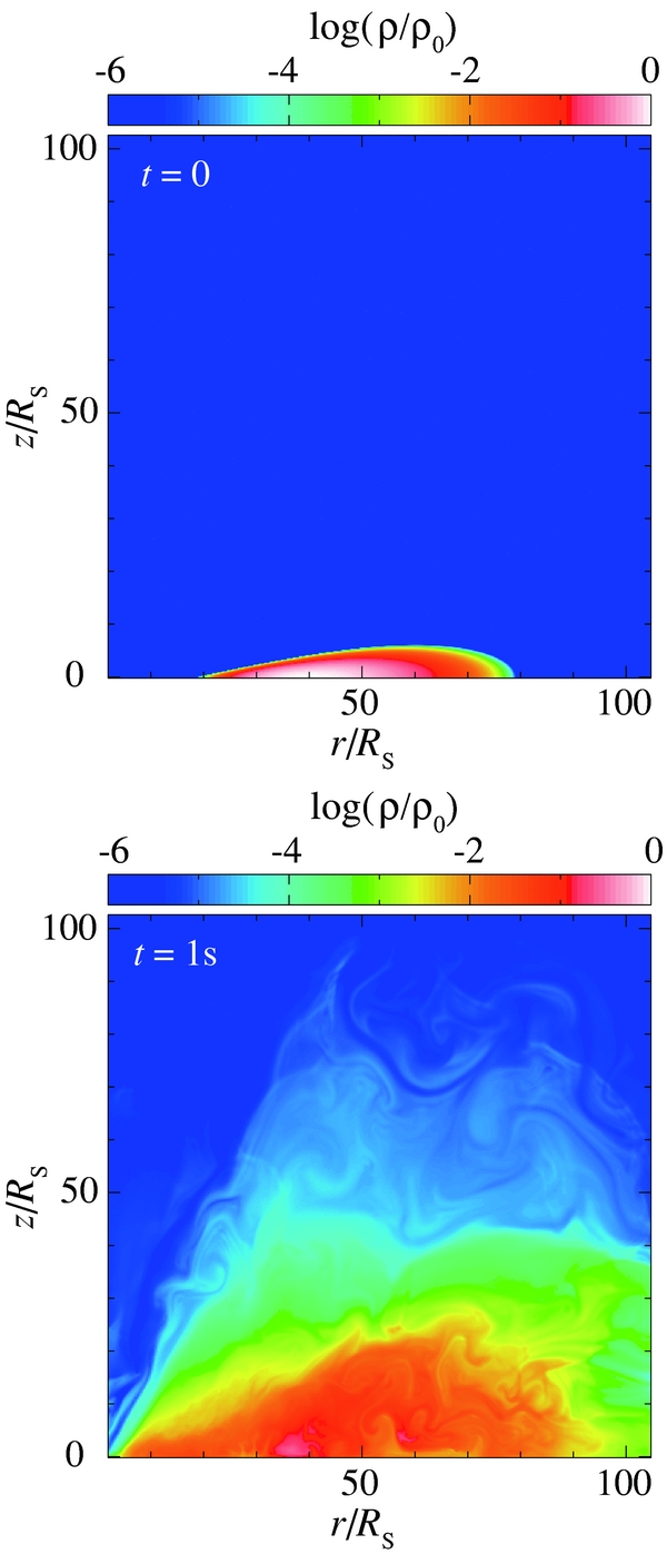
Figure 1. Color contour of the initial matter density distribution (top) and that obtained after 1 s non-radiative MHD simulations (bottom).
Download figure:
Standard image High-resolution image3.7. Mass Accretion Rates, Outflow Rates, and Luminosities
The mass accretion rate is calculated at the inner boundary at r = 2 RS by

which is the mass passing through the inner boundary per unit time. The photon luminosity is calculated by
at the height of z = zc. The values of (rc1, zc) are carefully chosen so as not to include the contribution from the initial torus. We, hence, set (rc1, zc) = (25 RS, 60 RS) for model A, (30 RS, 30 RS) for model B, and (60 RS, 60 RS) for model C. In model C we employ relatively larger rc1(= 60 RS); however, the contribution to the total emission from the outer region is very small, since the density is very small there. The mass outflow rate and the kinetic luminosity are also calculated at z = zc as


where H is the Heaviside step function; i.e., H(x) = 1 for x ⩾ 0 and H(x) = 0 for x < 0, and vR[ ≡ vr(r/R) + vz(z/R)] is the R-component of the velocity. We employ (rc2, zc) = (60 RS, 60 RS) for models A and C, and (rc2, zc) = (30 RS, 30 RS) for model B. That is, in the present study  and Lkin indicate the mass and kinetic energy transported upward only by the high-velocity outflow (vR > vesc) per unit time. In addition, we plot the luminosity of the trapped radiation, which is evaluated by
with r = 2 RS. It implies the radiation energy swallowed by the black hole per unit time.
4. RESULTS
We first give an overview of the simulation results in Section 4.1 and then provide more detailed information in Sections 4.2–4.4 for models A, B, and C, respectively.
4.1. Overview of Simulated Flows
The overall flow structures obtained by our RMHD simulations can be summarized in Figures 2–4. We first show perspective views of the simulated flows in models A−C in Figure 2. Here, the color contours indicate the distributions of normalized density, ρ/ρ0, time-averaged over 6–7 s for models A and C and over 9–10 s for model B. We find that a geometrically thick disk forms in models A and C, while a geometrically thin disk forms in model B. The streamlines indicated by the thick lines are overlaid in this figure. We find in all models that the gas near the equatorial plane is on a quasi-circular orbit around the central black hole, whereas the gas away from the equatorial plane shows helical and outflowing motion. The helical motion means that the outflow material possesses a substantial amount of angular momenta.

Figure 2. Perspective view of inflow and outflow patterns near the black hole for models A, B, and C, from left to right, respectively. Also plotted are normalized density distributions (color) and streamlines, which are time-averaged over 6–7 s for models A and C and over 9–10 s for model B.
Download figure:
Standard image High-resolution imageThe different dynamical properties of accretion flows in the three models are more quantitatively shown in Figure 3. In the top panel of the figure, we plot the normalized mass accretion rate,  ; mass outflow rate,
  ; photon luminosity, Lph/LE; kinetic luminosity, Lkin/LE; and trapping luminosity, Ltrap/LE. We also plot Lkin/Lph, Ltrap/Lph, and
  in the bottom panel. They are time-averaged over t = 5–7.5 s for models A and C and over 7.5–10 s for model B. For the calculation methods of these quantities, see Section 3.7.
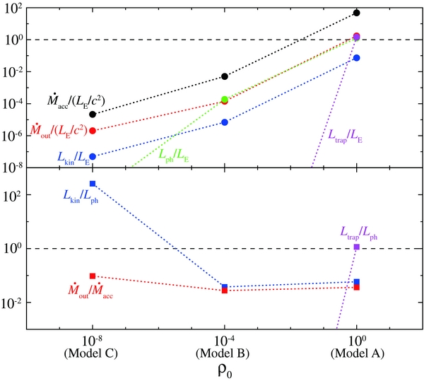
Figure 3. Top panel: mass accretion rate,  , and mass outflow rate,
  , normalized by the critical rate, LE/c2, and the photon, kinetic, and trapping luminosities normalized by the Eddington luminosity, LE. Bottom panel: the ratios of
  , Lkin/Lph, and Ltrap/Lph. All values are time-averaged over 5–7.5 s (models A and C) and 7.5–10 s (model B).
Download figure:
Standard image High-resolution imageWe find in model A that the photon luminosity exceeds the Eddington luminosity and that the trapping luminosity is substantial, implying that the model A flow is supercritical flow. The thin disk in model B corresponds to the standard-type disk, since low scale height is a result of efficient radiative cooling. By contrast, the photon luminosity is negligible in model C, indicating that the model C flow is RIAF. We also see a large value of Lkin/Lph (> 1) only in model C.
In Figure 4, we show the radial profiles of the density (top), the gas and radiation temperatures (middle), and the radial velocities (bottom) around the equatorial plane. They are time-averaged over t = 7.5–10 s. As expected, the gas temperature is highest in model C (RIAF), while it is lowest in model B except at radii less than ∼5 RS. The decoupling of the gas and radiation temperatures occur entirely in model C and inside ∼7 RS in model B.
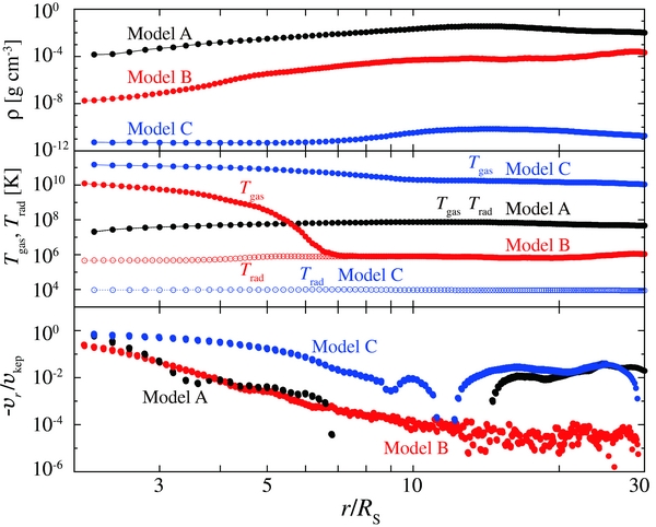
Figure 4. Radial profiles of the density (top), the gas and radiation temperatures (middle), and the inflow velocity normalized by the local Keplerian velocity (bottom) near the equatorial plane for models A (z = 0.1 RS, black), B (z = 0.05 RS, red), and C (z = 0.1 RS, blue). All values are time-averaged over 7.5–10 s.
Download figure:
Standard image High-resolution imageTo summarize, we could reproduce three distinct states of accretion flow with the same code by changing the density normalization. In the subsequent subsections we give more information individually for models A–C.
4.2. Model A
4.2.1. Overview
Model A, which has a high density normalization (ρ0 = 1.0 g cm−3), corresponds to the two-dimensional RMHD version of the slim disk model (Abramowicz et al. 1988; Watarai et al. 2000) but with significant outflow (Takeuchi et al. 2009). The geometrically thick disk is supported by radiation pressure (see Sections 4.2.2 and 4.2.3). We also find in Figure 4 that the disk consists of very dense and moderately hot (107–8 K) matter. The gas temperature is comparable to the radiation temperature due to the effective gas–radiation interaction. The inflow velocity (−vr) tends to increase inward only in the vicinity of the black hole, r ≲ 7 RS, and it is very small or even negative (i.e., outflow) around r ∼ 10 RS (see the bottom panel of Figure 4). The basic properties of model A are roughly consistent with those of the slim disk. However, the slopes of the radial profiles of the density and temperatures largely differ from those of the slim disk. (Note that such deviations from the conventional disk models are also found in models B and C.) These discrepancies might be due to the limited calculation time, the restricted computational domain, and the influence of the initial conditions. Detailed comparison is left for future work.
In Figure 3, we find that the mass accretion rate onto the black hole is much larger than the critical value,  . The photon luminosity is Lph ∼ 1.7LE, which is calculated based on the vertical component of the radiative flux within the polar angle of θ = tan −1(25 RS/60 RS) ∼ 23°. (Note that we assigned (rc1, zc) = (25 RS, 60 RS) in Equation (23).) Since (rc1, zc) = (25 RS, 60 RS) lies on the line of the photosphere, z/r ∼ 2.4 (see Section 4.2.2), the photon luminosity calculated with these values is equal to the sum of the radiation energy released at the photosphere of the inner part of the disk, r < 25 RS, per unit time. Also, since rc1 = 25 RS is smaller than the position of the initial torus, r = 40 RS, we can avoid possible influence by the initial conditions. Here we note that the calculated luminosity (Lph) may be underestimated, since the contribution from the outer disk (r ≳ 25 RS) was ignored. For better calculations of Lph, we need simulations with a larger computational domain, in which we set the initial torus at a much larger radius.
In addition, the photons mainly escape along the rotation axis, producing mildly collimated emission (note that the vertical component of the radiative flux is much larger than the radial one around the rotation axis, z/r > 2.4). Thus, the apparent luminosity of the flow would exhibit the strong viewing-angle dependence. We will discuss this issue in Section 5.
Figure 3 also indicates that the trapping luminosity is slightly larger than the Eddington luminosity (top panel), and is comparable to the photon luminosity (bottom panel). This means that the large number of photons generated inside the disk is swallowed by the black hole together with accreting matter, with many not being released from the disk surface.
Although we do not represent the rotation velocity in Figure 4, matter approximately rotates with Keplerian velocity (within 10%) near the equatorial plane. The outflow is driven by the radiation force (see Sections 4.2.2 and 4.2.3). The mass-outflow rate is a few percent of the mass accretion rate (see Figure 3). We also find Lkin ≲ 0.1Lph in this figure. This implies that the supercritical flows in model A release energy via radiation rather than via outflows.
4.2.2. Two-dimensional Structure
Figure 5 illustrates various aspects of the flow structure for model A. The contours of the density, the gas temperature, and the plasma-β are shown in panels (a), (b), and (c), respectively. Here, the velocity vectors are overlaid in panel (a) with arrows, in which the white arrows indicate that the velocity exceeds the escape velocity defined as vesc ≡ (2GM/R)1/2. The magnetic energies of the toroidal and poloidal components are separately plotted in panels (d) and (e), respectively, where the poloidal component is given by Bp = (B2r + B2z)1/2. The magnetic pitch, |Bφ|/Bp, is shown in panel (f). Panel (g) indicates the radiation energy, and the ratio of the radiation energy to the sum of the gas and magnetic energies is plotted in panel (h). Panel (i) shows the ratio of the gas temperature to the radiation temperature, where the radiation temperature is calculated as Trad = (E0/ar)1/4. All values are time-averaged over t = 6–7 s, and both axes are normalized by the Schwarzschild radius.
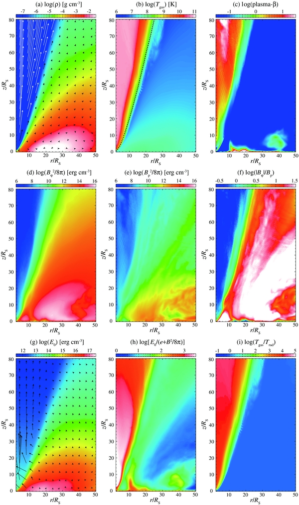
Figure 5. Two-dimensional distribution of the various quantities for Model A: (a) the density overlaid with the velocity vectors, (b) the gas temperature, (c) the plasma-β, (d) the magnetic energies via the toroidal component of field, (e) the same but of the poloidal component, (f) the magnetic pitch, (g) the radiation energy, (h) the ratio of the radiation energy to the sum of the gas and magnetic energies, (i) and the ratio of the gas temperature to the radiation temperature. All values are time-averaged over t = 6–7 s The white and black arrows in panel (a) indicate the velocity vectors whose magnitude exceed the escape velocity. The dashed line in panel (b) is the photosphere, at which the optical thickness measured from the upper boundary is unity. The arrow in panel (g) shows the radiative flux vector.
Download figure:
Standard image High-resolution imageWe find in panel (a) that the flow is divided into two regions: the disk region around the equatorial plane (characterized by white and red colors) and the outflow region above the disk region (blue region). The boundary between the two regions is approximately along the line of z/r ∼ 2. The matter slowly accretes onto the black hole through the disk region with velocity much less than the free-fall velocity (small black arrows). This panel also shows that the outflow velocity greatly exceeds the escape velocity (white arrows). The photosphere, at which the optical thickness measured from the upper calculation boundary is about unity, roughly corresponds to the green region, i.e., z/r ∼ 2.4.
We find that the hot, rarefied corona appears above the supercritical disk. Panel (b) indicates that the outflowing matter is very hot (≳ 109 K), whereas the disk consists of relatively hot gas (∼107–8 K). The gas density is much smaller in the outflow region than in the disk region (see panel (a)). Such a hot outflowing corona above the supercritical disk has also been reported by Ohsuga et al. (2005b) and is thought to affect the spectra due to Comptonization (Kawashima et al. 2009).
Panel (c) shows that the outflow is surrounded by a low plasma-β region (blue), in which we find plasma-β <1. In such a low plasma-β region, the toroidal component of the magnetic fields, which seems to be amplified via the differential rotation of gas, dominates over the poloidal one (see panels (d) and (e)). This feature is also clearly demonstrated in panel (f), in which we see |Bφ|/Bp > 10 around the outflow region. That is, the outflow is surrounded by regions with strong toroidal magnetic fields. Inside the outflow, on the other hand, the vertical component of the magnetic fields dominates over the other components.
Such a magnetic structure is quite reminiscent of magnetic-tower jets (Lynden-Bell & Boily 1994; Lynden-Bell 1996; Kato et al. 2004b). However, there is one big difference: while the magnetic tower jets are accelerated via magnetic-pressure force, the outflow in our model A is powered by radiation force. This radiatively driven outflow is collimated by the Lorentz force. Thus, on the basis of global RMHD simulations we propose a novel jet model: the radiation-pressure driven and magnetically collimated outflow (see also Takeuchi et al. 2010).
Note that there must be something preventing the field from expanding sideways, thereby giving rise to the high magnetic energy density in the cylindrical region around the black hole. In our simulations it is the radiation-pressure force from the geometrically thick flow surrounding the magnetic tower that confines the magnetic tower. The magnetic field can thus naturally evolve from its initial configuration to form such a high concentration (Takeuchi et al. 2010).
In panel (g), it is found that the radiation energy is enhanced in the disk region. The disk is not only geometrically thick but also optically thick. Because of numerous scatterings, the photons generated in the disk cannot easily escape from the disk surface. As a consequence, a large number of photons accumulate in the disk region, leading to the high radiation energy density. The radiation energy predominates over the gas energy, and also over the magnetic energy in the entire region (see panel (h)). The ratio of the radiation energy to the sum of the gas and magnetic energies is ≳ 103 in the outflow region and ≳ 10 in the disk region.
Panel (i) indicates that the gas temperature is nearly equal to the radiation temperature within the disk (blue). The absorption opacity is large in the disk region, since it is sensitive to the density (∝ρ2). Thus, the effective gas–radiation interaction (emission/absorption) leads to Tgas ∼ Trad. In contrast, the gas temperature is much higher than the radiation temperature in the outflow region, where the radiative cooling is not efficient because of the small absorption opacity (small density). Thus, the gas temperature is kept high (see the next subsection for more quantitative descriptions).
4.2.3. Vertical Structure
In the top panel of Figure 6, we plot the vertical profiles of the density (red) and the vertical component of the velocity (black) for r/RS = 10. Here, they are time-averaged over t = 5–7.5 s. We find that the density decreases as z increases. The upward velocity increases as z increases and it exceeds the escape velocity at z ≳ 20 RS. The sonic point is around z = 20 RS. While the gas temperature is comparable to the radiation temperature due to the effective gas–radiation interaction at z ≲ 15 RS, we find Tgas ≫ Trad at the upper region of z ≳ 20 RS, since radiative cooling is inefficient because of smaller density (emissivity; see the middle panel).
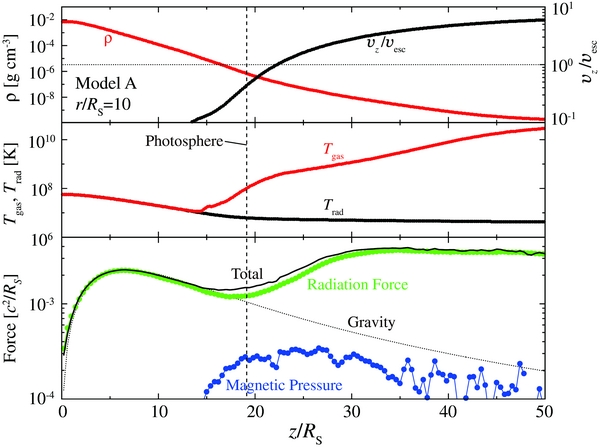
Figure 6. Vertical structure at r = 10 RS for model A. Top panel: the density (red) and vertical component of the velocity normalized by the escape velocity (black). Middle panel: the gas and radiation temperatures. Bottom panel: the vertical components of the gravity (dotted line), the radiation force (green filled circle), and the magnetic-pressure force (blue filled circle). The sum of the vertical forces due to the radiation, the magnetic pressure, the magnetic tension, and the gas pressure is plotted by the black solid line (total). Here, the gas-pressure force (red filled circle) and the magnetic-tension force (blue open circle) are not represented, since they are so small or negative. All values are time-averaged over 6–7 s.
Download figure:
Standard image High-resolution imageAs we have mentioned in Section 4.2.2, the supercritical disk ejects high-velocity outflows driven by the radiation force. This is clearly shown in the bottom panel of Figure 6, in which we plot vertical components of the gravity (dotted line), the radiation force (green circle), and the magnetic-pressure force (blue circle). The solid black line (total) in the bottom panel indicates the sum of the vertical forces from the radiation, the magnetic pressure, the magnetic tension, and the gas pressure. (The gas-pressure force and the magnetic-tension force are so small that they do not appear in this figure.) While the radiation force is nearly balanced with the gravity at z ≲ 20 RS (disk region), it largely exceeds the gravity in the upper regions at z ≳ 20 RS, producing the high-velocity outflows. The radiative flux is roughly estimated to be cE0 in the optically thin, outflow region above the disk, whereas it is reduced to be cE0/τ in the optically thick disk region. Hence, the radiation force suddenly increases above around the disk surface, z ∼ 20 RS, although the radiation energy density itself (E0) is smaller in the outflow region than in the disk region (see panel (g) of Figure 5). In the case of supercritical flows, the radiation force supports the disks and accelerates the outflows. The forces via the magnetic pressure, the magnetic tension, and the gas pressure is too small to influence the acceleration of the outflow. However, the magnetic pressure and the magnetic tension (Lorentz force) works in a direction parallel to the disk plane and thus collimates the outflow (see Takeuchi et al. 2010).
4.2.4. Dissipation Rate
In Figure 7, we plot the vertical profiles of the dissipation rate, 4πηJ2/c2 (black), as well as those of the gas (red), radiation (green), and magnetic energies (blue) for model A (see upper four lines). They are time-averaged over 5–7.5 s. All the values tend to decrease with an increase of z. In the region of z ≲ 20 RS, we find that the gradient of the dissipation rate is smaller than that of the gas energy and that of the radiation energy. It implies that the traditional α-viscosity model does not precisely describe the vertical structure of the disk, since it states that the dissipation rate is proportional to the gas (or radiation) pressure. We find that the profile of the dissipation rate is roughly parallel with that of the magnetic energy (see also Turner et al. 2003; Hirose et al. 2006 for the cases of local RMHD simulations).
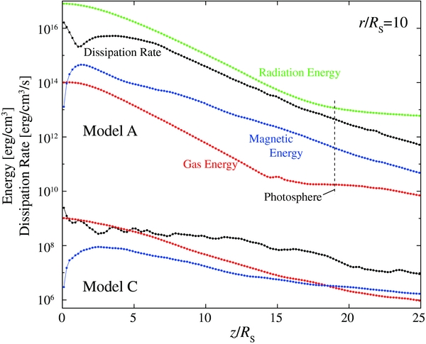
Figure 7. Vertical profiles of the energy dissipation rate (black), and the gas (red), radiation (green), and magnetic (blue) energies at r = 10 RS. They are time-averaged over 5–7.5 s The radiation energy in model C is not plotted, since it is too small.
Download figure:
Standard image High-resolution imageThe radiation energy shows a rather flat distribution above z ≳ 20 RS. Since the radiation energy is transported via diffusion in the disk region, while the photons freely go out above the disk, the slope of the radiation energy profile changes across the disk surface at z ∼ 20 RS.
In Figure 7, we also find that, while the dissipation rate is enhanced near the equatorial plane in both models, the magnetic energy suddenly decreases toward z = 0. However, caution should be taken here, since this might be caused by the particular boundary conditions with respect to the equatorial plane, where we require that Br and Bφ are antisymmetric. Such a condition enhances reconnection, leading to a decrease in the magnetic energy and an increase in the dissipation rate. In fact, Hirose et al. (2006) showed by simulations that the magnetic energy and the dissipation rate are nearly constant across the equatorial plane without employing the equatorial-plane symmetries.
Although the traditional α-viscosity model does not precisely describe the vertical dissipation profile, the r–φ component of the shear-stress tensor around the equatorial plane is roughly proportional to the pressure when we examine the time variations of these two quantities. In our previous paper (Ohsuga et al. 2009), we investigated the time evolution of the magnetic torque of z ≲ 3 RS, and demonstrated that the torque is roughly proportional to the total pressure but with some scattering.
4.2.5. Gaussian or Polytropic?
Finally, we compare the simulated vertical structure with that obtained by simple analytic models on the assumption of hydrostatic balance. If the disks are vertically isothermal, the energy (pressure) profile is given by a Gaussian profile of exp (− z2/2H2) with H being the disk half-thickness. Such a function with H = 2.5 RS roughly reproduces the energy distributions of the flow in model A, as is seen in the top panel of Figure 8, which represents gas and radiation energies of model A normalized by the values at z = 0. If we use a polytropic relation (p∝ρ(N + 1)/N with N being the polytropic index) instead of the isothermal assumption, the vertical hydrostatic balance leads to the energy being proportional to a function of (1 − z2/2H2)N + 1. Such a function with H = 8 RS can also give good fits to the energy profiles of model A (see the upper panel in Figure 8). Here, we employ N = 3 for model A since the disk is radiation-pressure-dominated. We note that the disk half-thickness at r = 10 RS is H ∼ (cS/vKep)r ∼ 5 RS and are in rough coincidence with the above values, where cS is the sound velocity at (r, z) = (10 RS, 0).

Figure 8. Gas and radiation energies of model A (top) and gas energy of model C (bottom) normalized by each value at z = 0. Solid and dotted lines indicate the Gaussian and polytropic relations, respectively.
Download figure:
Standard image High-resolution image4.3. Model B
4.3.1. Overview
As already mentioned, accretion flows at r ≳ 7 RS in our model B (ρ0 = 10−4 g cm−3) resemble the standard disk. The efficient radiative cooling leads to the formation of a geometrically thin but optically thick disk (see Figure 2). The disk in model B is moderately dense as shown in the top panel of Figure 4. The gas temperature of ∼106K at r ≳ 7 RS is close to the value predicted by the standard disk model (see the middle panel of Figure 4). However, the disk is truncated around r ∼ 7 RS (which we call the truncation radius). Because of the small density of the accretion flow near the black hole, the emissivity is greatly reduced, which is responsible for the decoupling of the gas and radiation temperatures, Tgas ≫ Trad at r ≲ 5 RS. The bottom panel shows that the inflow velocity (−vr) increases as the flow approaches the black hole. The rotation velocity is very close to the Keplerian velocity (within 10%), although we do not represent it in Figure 4.
We find in Figure 3 that the photon luminosity is well below the Eddington luminosity, ∼2 × 10⁻⁴LE, for the mass accretion rate is ∼5 × 10⁻³LE/c2. In this model, the photon trapping effect is negligible. The energy conversion efficiency,  , is the largest in the three models. This is also consistent with the prediction of the one-dimensional accretion disk study, whereby radiative cooling is more effective in the standard disk model than in the slim disk model and RIAF. However, the simulated value of η is smaller than the prediction of the standard disk model, ∼0.1. This result might be caused by the disk truncation around r ∼ 7 RS, within which the density is too small for emission to be efficient (this will be discussed in Section 5.2). If we were to employ higher density normalization, both the photon luminosity and the conversion efficiency might increase, since the truncation radius would then decrease or even disappear. Such a disk would be more consistent with the standard disk model.
Whereas disk wind is not predicted by the standard disk model, a significant amount of matter is blown away in model B. As we have already mentioned in Section 4.1, the matter above the disk rotates and moves upward. In other words, outflow material possesses substantial angular momentum, taking it away from the underlying disk. Figure 3 shows that the time-averaged mass-outflow rate is about 10−4LE/c2 (see the top panel), which is a few percent of the mass accretion rate (see the bottom panel). We also find in the bottom panel that Lkin is a few percent of Lph. As is the case in model A, the disk in model B releases energy via radiation rather than via outflows. Here we note a possibility that the outflowing matter with high velocity might originate not from the cold outer part of the disk (r ≳ 7 RS) but from the hot inner part of the disk (r ≲ 5 RS). The matter ejected from the cold outer part of the disk might produce low-velocity outflow with a wide opening angle. At this moment it is technically very difficult to identify the launching points of the high- and low-velocity outflows. Note that there is no clear evidence for the collimation of the outflows in model B.
4.3.2. Two-dimensional Structure
The two-dimensional structure of the flow in model B is presented in Figure 9. Each physical quantity is time-averaged over t = 9–10 s. Panel (a) clearly shows that a geometrically thin disk is located around the equatorial plane (indicated by the white and red colors). The disk thickness is very small and is everywhere less than ∼1 RS. The gas of the disk effectively cools by emitting radiation, as shown in panel (b), except at r ≲ 5 RS. The gas temperature is very high above and below the disk, since the low density leads to a low cooling rate (emissivity). Such a high-temperature and low-density matter forms a corona surrounding the cold disk and Compton upscatters seed photons generated within the scale height of the disk.

Figure 9. Same as Figure 5 but for model B. Each quantity is time-averaged over t = 9–10 s Note the different plot area from that of Figure 5.
Download figure:
Standard image High-resolution imagePanel (c) shows that a relatively low plasma-β region appears along the line of |z|/r ∼ 2 (green and light blue). We find that the matter goes upward in this region (see the vectors in the blue region in panel (a)). Although the time-averaged velocities are less than the escape velocity, the upward velocity intermittently exceeds the escape velocity. As a result, the time-averaged mass-outflow rate is  (see Figure 3). Panel (f) shows that this outflow is surrounded by the regions of |Bφ|/Bp > 1, while the poloidal (vertical) component of the magnetic fields dominates at the very vicinity of the rotation axis. These features can be seen in panels (d) and (e). The toroidal field is enhanced mainly near the disk, |z| ≲ 10 RS (see panel (d)). The poloidal component, in contrast, tends to be enhanced near the black hole (see panel (e)). Again, a magnetic-tower-like structure appears in model B as well. Here we note that the higher plasma-β and the larger magnetic pitch at the outer region (r ≳ 20 RS and |z| ≲ 15 RS) are thought to be under the influence of the initial torus.
We find in panel (g) that the radiation energy is enhanced within the disk (white and red), since the disk is optically thick except at r ≲ 7 RS. The optical thickness of the disk atmosphere is, by definition, smaller than unity, implying that the photons emitted at the disk surface can freely go out. Thus, the radiation energy is small above and below the disk (blue). In contrast with model A, the radiation energy is smaller than the gas energy and the magnetic energy (see panel (h)).
Panel (i) shows Tgas ∼ Trad in the disk at r ≳ 7 RS (blue), and Tgas ≫ Trad in the other regions (white and red). This is because the gas–radiation interaction is effective only in the dense region as we have already mentioned. Such a feature is similar to that in model A, though the disk is geometrically thin in model B.
4.3.3. Vertical Structure
Figure 10 is the same as Figure 6 but for model B and t = 7.5–10 s. In the bottom panel, the red circles indicate the gas-pressure force. In the top panel, the high-density regions of z < RS correspond to the thin disk as we have shown in Figure 9. The density slowly decreases with an increase of z above the disk. This is because the gas temperature and the scale height are very high in the low-density region at z > RS (middle panel). We find Tgas ∼ Trad in the disk region.
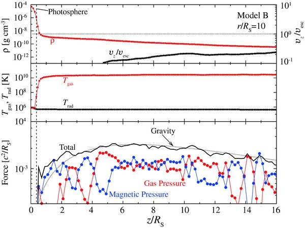
Figure 10. Same as Figure 6 but for model B. Each quantity is time-averaged over t = 9–10 s Here, the radiation force (green filled circle) and the magnetic-tension force (blue open circle) are not represented, since they are so small or negative. Here we note that the disk region contains 5–6 grid points (excluding the point at the boundary). Although this number is not big, it can marginally resolve the vertical structure.
Download figure:
Standard image High-resolution imageWe find that sum of the gas and magnetic-pressure forces roughly balance with the gravity at z ≳ 3 RS (see the bottom panel). The time-averaged upward velocity is much smaller than the escape velocity in this region (see the top panel). Note, however, that the high-velocity outflows occasionally appear.
How is the matter ejected from the disk? It is mainly by the magnetic-pressure force. The bottom panel shows that the hydrostatic balance breaks down around the disk surface, z = 1–3 RS, where the magnetic-pressure force exceeds the gravity, leading to mass ejection from the disk surface. In contrast with model A, the radiation force is negligible.
Although we used small grid spacings, Δr = Δz = 0.1 RS, in our simulations for model B, we note that the simulations of even higher resolution are required to investigate the detailed structure of the geometrically thin disk. Such calculations will be performed in a future study.
4.4. Model C
4.4.1. Overview
Flows in model C (ρ0 = 10−8 g cm−3) correspond to RIAF. The geometrically thick disk is supported by gas pressure together with the magnetic pressure (see Sections 4.4.2 and 4.4.3). As shown in Figure 4, the flow is entirely occupied by very hot and rarefied plasma. Since the density is too low for radiative cooling to be effective, a decoupling of the gas and radiation temperatures, Tgas ≫ Trad, occurs in the whole region. The bottom panel in Figure 4 shows that the accretion velocity is relatively high at r ≲ 10 RS in comparison with those of the flows in models A and B.
Since the optical thickness is very small (τ ∼ 10−4), the flow in model C is radiatively inefficient and faint. The photon luminosity is much smaller than the Eddington luminosity, Lph ≪ 10−8LE (see Figure 3). The energy conversion efficiency in model C (η ∼ 10−5) is much smaller than those in models A and B.
The helical streamlines seen in Figure 2 indicate the formation of jets around the rotation axis. The mass-outflow rate is about 10 % of the mass accretion rate (see Figure 3). Interestingly, we find Lkin > 102Lph in model C (cf. Lkin < 0.1Lph in models A and B). Hence, the radiatively inefficient disk ( ) loses the energy more via jets rather than via radiation.
4.4.2. Two-dimensional Structure
Figure 11 shows the two-dimensional structure of the flow in model C. This figure is the same as panels (a)–(f) of Figure 5 but for model C. The white and red colors in panel (a) indicate a geometrically thick disk (disk region). The entire zone can be divided into the disk and outflow regions by the z/r ∼ 2 line. The gas temperature greatly exceeds 109 K in the whole region (panel (b)). Here we note that we might overestimate the gas temperature, since cooling via Compton scattering is not taken into consideration. Also, the electron temperature might deviate from the ion temperatures, although we treat the matter as a one-temperature plasma. The disk is mainly supported by the gas pressure. The gas energy dominates over the magnetic pressure in the disk region (see panel (c)).

Figure 11. Same as panels (a)–(f) of Figure 5, but for model C. Here, note that there is no photosphere, since the flow is optically thin.
Download figure:
Standard image High-resolution imageIn panel (a), we also find that matter with relatively small density is blown away above the disk, i.e., z/r ≳ 2. (The outflow region is defined by the green and yellow colors.) The time-averaged outward velocity exceeds the escape velocity only in the region of z ≳ 70 RS in panel (a) (white vectors). Note, however, that this figure only shows the time average, while the simulations exhibit significant time variations in vR. In fact, we find that the high-velocity outflows (vR > vesc) occasionally appear at z ≳ 10 RS near the rotation axis. The outflow is mainly accelerated via magnetic pressure, in concert with the gas pressure (see discussion below). The radiation force is negligible.
Panel (c) indicates the plasma-β ≲ 1 in the outflow region, whereas β > 1 in the disk region. The toroidal magnetic fields are mainly amplified in the disk region, while poloidal fields strengthen around the rotation axis (see panels (d) and (e)). Hence, the magnetic pitch, |Bφ|/Bp, tends to increase as r increases. Panel (f) shows that the pitch becomes large around the outer edge of the outflow region located along the z/r ∼ 2 line (see the yellow area). This implies that the magnetic field lines are strongly coiled around the spine of the outflow, that is, helical magnetic fields form. Thus, the outflow in model C seems to be magnetic tower jets, which have been reported in the three-dimensional MHD simulations by Kato et al. (2004b; see also Lynden-Bell & Boily 1994; Lynden-Bell 1996, for the original proposal).
Since the disk is optically thin, the photons can freely escape from the disk, producing a quasi-spherical distribution of the radiation energy density, as clearly shown in panel (g). Again, the radiation force is negligible due to the small radiation energy and small opacity.
4.4.3. Vertical Structure
Figure 12 is the same as Figure 6 but for model C. The density and the gas temperature monotonically decrease as z increases. The open blue circles indicate the vertical component of the magnetic-tension force. We find that the geometrically thick disk at z ≲ 20 RS is mainly supported by gas pressure, achieving hydrostatic balance (see the bottom panel). The magnetic-pressure force dominates over the gas-pressure force above the disk, z ≳ 20 RS. In this region, the total force (black line) exceeds the gravity, implying that matter is accelerated upward. That is, the magnetic-pressure force, together with the gas-pressure force, drives the outflows above and below the disk. The outflow is thus accelerated upward; its velocity exceeds the sound velocity at z ∼ 30 RS and reaches the escape velocity at z ∼ 50 RS. Both the radiation force and the magnetic-tension force are found to be negligible.

Figure 12. Same as Figure 6 but for model C. Here, the radiation force (green filled circle) is not shown, since they are negligibly small. Note that the gas pressure exceeds the total pressure at small heights, z ⩽ 2 RS (see the bottom panel). This is because the vertical force by the magnetic pressure is negative there.
Download figure:
Standard image High-resolution imageSimilarly to model A (see Figure 6), we find in model C that the disk is in hydrostatic balance and matter is blown away from the disk surface. However, the radiatively driven outflows in model A are more powerful than the magnetically driven outflows in model C. (The kinetic luminosity, Lkin, is larger in model A than in model C.) While the radiation force largely exceeds the gravity in model A, the upward force only slightly exceeds the gravitational force in model C (see the bottom panel in Figure 12). As a result, low-luminosity disks with  cannot produce powerful high-velocity outflows continuously, but only occasionally.
4.4.4. Dissipation Rate
The three lower lines in Figure 7 represent the vertical profiles of the dissipation rate (black), and gas (red) and magnetic energies (blue) for model C, which are time-averaged over 5–7.5 s. Here, we note that the radiation energy is negligible in model C, so it is not plotted. We find that the slope of the profile of the dissipation rate is nearly equal to that of the magnetic energy, and flatter than that of the gas energy. Such a feature implies that the traditional α-viscosity model does not precisely describe the vertical flow structure, as already noticed in model A. As we have discussed in Section 4.2.4, the boundary condition with respect to the equatorial plane seems responsible for the enhanced dissipation rate, leading to the drop of the magnetic energy at z ∼ 0.
4.4.5. Gaussian or Polytropic?
In Section 4.2.5, we have mentioned that the energy distributions of the flow in model A agrees with the profiles of the disks in hydrostatic balance (isothermal and polytropic). However, we cannot fit the profile of the gas energy of model C by the Gaussian profile (with H = 3 RS) nor by the polytropic relation (with H = 7 RS; see the bottom panel in Figure 8). Here, N = 1.5 is used because the gas pressure is predominant for the disk of model C. Even if we change H, the fitting is not successful. The drop of the gas energy is more rapid at small z (≲ 4 RS) and steeper above this value. Such deviations may be caused by the particular magnetic energy profile which is not simply proportional to gas pressure. Finer-mesh calculations are necessary to confirm if this is really the case.
5. DISCUSSIONS
5.1. Comparison with Observations: Outflow
Our simulations demonstrate that powerful outflows appear in the super- or near-critical flows (model A). This result seems to be consistent with the observations of bright black hole objects with high Eddington ratio, such as narrow-line Seyfert 1 galaxies (NLS1s) and microquasars. The NLS1s, which are thought to contain relatively less massive black holes and thus to be high Lph/LE systems, are usually radio-quiet. However, some of them have been reported to be radio-loud. Doi et al. (2006), for example, concluded by very long baseline interferometry observations that a radio-loud NLS1, J094857.3+002225, possesses relativistic jets (see also Zhou et al. 2003). By contrast, there are plenty of such sources in our Galaxy. Microquasars, such as GRS 1915+105, also show relativistic jets in high-luminosity state (Fender et al. 2004) and SS433 is another good example of supercritical accretion flow with powerful jets.
Model A may explain the nebulae (or bubbles) around ultraluminous X-ray sources (ULXs) or microquasars. Pakull et al. (2010) proposed, using X-ray/optical observations, that the large nebula S26 is produced by energy injection via powerful jets, of which the kinetic luminosity is estimated to exceed the photon luminosity, Lkin > Lph, by three orders of magnitude (see also Pakull & Grisé 2008). The supercritical flows will be observed as low-luminosity objects (Lph < Lkin) near the edge-on view, since the emission is mildly collimated and since the radiation from the innermost region can be obscured by the outer disk. If this is the case, the large Lkin/Lph ratio of S26 can be explained by model A. By solving the radiation transfer equation, Ohsuga et al. (2005b) demonstrated that the apparent luminosity in the edge-on view could be more than 10 times smaller than that in the face-on view. In this calculation, large luminosity comes from the middle part of the disk at r ≳ 100 RS due to the limitation of the computational box. If we can make simulations with a much more extended computational box, an even smaller value of Lph is expected at the edge-on view. Since Lkin is on the order of LE regardless of the viewing angle, the large Lkin/Lph is, hence, expected.
Model B exhibits disk wind and a geometrically thin disk, which were not predicted in the framework of the standard disk model. The recent X-ray observations of black hole binaries (BHBs) reveal the presence of the blueshifted absorption lines, indicating the occurrence of disk wind from a geometrically thin disk. Miller et al. (2006a, 2006b) concluded, using the observations of GRO J1655-40 and a black hole candidate, H1743-322, that matter with ρ ∼ 10−9 g cm−3 was ejected from the geometrically thin disk with the speed of 500–1600 km s−1. The outflow velocity of the X-ray transient, 4U 1630-472, has been also reported to be ∼103 km s−1 (Kubota et al. 2007). The present study can account for such observations. Model B shows that the gas with ρ ∼ 10−9 g cm−3 goes out at the speed of ∼103 km s−1 (see Figures 9 and 10).
We find a magnetic tower jet in model C. In contrast with models A and B in which we find Lkin < Lph, the kinetic luminosity largely exceeds the photon luminosity in model C, Lkin ≫ Lph (see Figure 3). That is, the radiatively inefficient flow releases energy mainly via the jet. This result can be understood through the predictions, whereby the kinetic luminosity is proportional to the mass accretion rate,  , but
, but  in the radiatively inefficient regime (Fender et al. 2004; Narayan & Yi 1995; Kato et al. 2008; see also Figure 3).
5.2. Comparison with Observations: Spectra
Model A might resolve the outstanding issue regarding the central engine of ULXs. As for their central engines, two competing models have been discussed over the past decade: subcritical accretion onto intermediate-mass black holes with the black hole mass greatly exceeding 100 M☉ (e.g., Makishima et al. 2000; Miller et al. 2004) and supercritical accretion onto stellar-mass black holes with mass of 3–20 M☉ (e.g., King et al. 2001; Watarai et al. 2001). In addition, there is the possibility that some ULXs may be powered by stellar (but not stellar-mass) black holes in the 30–80 M☉ range, formed in low metallicity environments, with near-critical or slightly supercritical accretion flows (e.g., Zampieri & Roberts 2009; Mapelli et al. 2010; Belczynski et al. 2010). It is thus crucially important to show theoretically how much (apparent) luminosity can be achieved by supercritical accretion.
The photon luminosity in model A is calculated based on the radiative flux mildly collimated within the polar angle of θ = tan −1 (25 RS/60 RS) ∼ 23° as we have mentioned in Section 4.2.1. Hence, the flows in model A would be identified as extremely luminous objects of ∼13Lph = 22LE for the accretion rate of ∼300LE/c2, or 1.5 × 1041 erg s−1, for the case of a black hole of 50 M☉, in the face-on view, if an observer assumes isotropic radiation field. Even higher apparent (isotropic) luminosities are feasible for higher accretion rates, since there is practically no limit to the mass accretion rate (Ohsuga 2006).
The outflowing matter in model A is very hot, Tgas ≳ 109 K, and dense, τes ∼ 1, with τes being the Thomson scattering optical depth, while the disk is relatively cold, Tgas ∼ 107–8 K (see Figures 5 and 6). Thus, the hot outflowing matter would Compton upscatter photons from the disk surface. Kawashima et al. (2009) have shown that at high luminosities, Lph ≳ LE, a very hard spectral state appeared due to the effective inverse Compton scattering by the radiatively driven outflow. Their result can explain the hard X-ray spectra of ULXs (e.g., Berghea et al. 2008) and seems to correspond to the ultraluminous state of ULXs (Gladstone et al. 2009). In addition, since an inner part of the disk is obscured by the strong outflow, the hot thermal component might be invisible. Indeed, Gladstone et al. (2009) have concluded based on X-ray observations that the strong outflow envelops the inner part of the supercritical disk, producing the cool spectral component in some ULXs. Optically thick (τes ≳ 3) low temperature (∼10 keV) corona are observed both in GRS 1915+105 and ULX Holmberg IX X-1 (Vierdayanti et al. 2010a, 2010b).
The geometrically thin, cold disk in model B is surrounded by hot and rarefied matter (Figure 9). Thus, the hot electrons in the corona would Compton upscatter the seed photons from the cold disk. While the thermal component of the spectra in active galactic nuclei (AGNs) and BHBs is thought to be of disk origin, the Compton upscattering in the corona can account for the non-thermal hard component (Deufel & Spruit 2000; Liu et al. 2003; Done & Gierliński 2004, 2005). No such extended disk corona was reproduced by simulations of the local patch of the disk, which only show small, hot spots (with Tgas ∼ 108 K) appearing near the disk surface (Hirose et al. 2006).
In the model B simulation, the optically thick, geometrically thin disk is truncated around r ∼ 7 RS (see Section 4.3.1). Such a disk truncation has been reported by recent observations (Kubota & Done 2004; Tomsick et al. 2009; Yamada et al. 2009) and by theoretical spectral modeling (Kawabata & Mineshige 2010). Blackbody radiation cannot be emitted within the truncation radius, but instead the seed photons generated in the cool outer disk will be Compton upscattered by the hot electrons in the inner region. It then follows that the iron line is produced not at the innermost stable circular orbit but at the inner edge of the cool disk (truncation radius). If so, it would be difficult to derive information about the black hole spin (Done & Gierliński 2006).
Note, however, that evaporation of the disk gas due to thermal conduction is not taken into account in the present simulation, although it could be an important ingredient in disk truncation (see Section 9.2.3 of Kato et al. 2008 for a comprehensive discussion).
The disk in model C is optically thin and is composed of hot rarefied plasma. Synchrotron self-absorption, synchrotron self-Compton, and free–free emission should be the dominant radiative processes (Liu et al. 2003; Ohsuga et al. 2005a; Kato et al. 2009). Such spectra are observed in low-luminosity AGNs and in the low–hard state of BHBs. Sgr A* is also a good example. Note that the electron temperature has been reported to deviate from the ion temperature (Narayan & Yi 1995; Nakamura et al. 1996; Manmoto et al. 1997), although we assume a one-temperature plasma in the present study. The emission of nonthermal electrons is thought to be non-trivial (Yuan et al. 2003). More detailed study is, however, beyond the scope of this paper.
5.3. Future Work
Global RMHD simulation is a relatively new research field and so there are plenty of issues to be explored in future work. We stress again that higher resolution simulations are needed to study the detailed structure of the geometrically thin disk as in model B. Three-dimensional simulations should also be explored in future work. It is well known that no magnetic dynamo works in axisymmetric calculations. Hence, three-dimensional simulations are indispensable to make progress. We also stress that it is better to relax reflection symmetry with respect to the equatorial plane, since such a symmetry prevents the flows from going across the equatorial plane. We plan such simulations for future work. In addition, we should take into account the relativistic effects, since the outflow velocity becomes 10%–70% of the speed of light near the rotation axis. In the present work, we begin calculations with a rotating torus, in which the magnetic fields are purely poloidal. We should investigate the inflow–outflow structure starting with other initial conditions in future.
We used the FLD technique in the present study. This is quite a useful technique and gives appropriate radiation fields within the optically thick disk, but we should keep in mind that it does not always give precise radiation fields near the disk surface and above the disk (where the optical depth is around unity or less). In order to investigate the validity of the FLD, we calculate accurate radiative flux (RT flux) by solving the radiation transfer equation along 104 light rays at some points. The resulting RT flux is presented by a white vector in Figure 13, where the RT flux evaluated based on the FLD method (FLD flux) is overlayed by a black vector. Here we employ a time-averaged (6–7 s) structure of model A, since the radiation force (RT flux) in this model plays important roles. We find in this figure that the FLD flux shifts from the RT flux in the outflow regions and near the photosphere, although the FLD flux is almost equal to the RT flux in the optically thick disk regions. In particular, the radial component of the FLD flux is negative (inward flux), but, in contrast, that of the RT flux is positive (outward flux; e.g., see the fluxes at r ∼ 7 RS with z ∼ 12Rs). The radiation from the vicinity of the black hole works to produce the outward RT flux. However, the inward flux appears by the FLD method, since the direction of the flux is determined by the gradient of the radiation energy density. Thus, we should employ a more accurate method for the radiation fields in the future. One of the improved methods is the so-called M1 closure scheme (González et al. 2007). In this method, the 0th and 1st moment equations of radiation transfer are solved to update the radiation energy and the radiative flux. A closure relation, which is used to evaluate the radiation pressure tensor, is described in terms of the radiation energy and radiative flux. (In the FLD approximation, by contrast, the radiation pressure tensor is prescribed by the radiation energy only, and no information regarding radiative energy flux is used. This may result in a somewhat inaccurate evaluation regarding the direction of radiation force in the jet acceleration region.)

Figure 13. Radiative flux vectors by FLD approximation (black; FLD flux) and by integrating the radiation intensity (white; RT flux). Here, we solve the radiation transfer equation along 104 light rays at each point for RT flux. Color contour indicates the radiation energy density, and the photosphere is plotted by the dashed line.
Download figure:
Standard image High-resolution image
Throughout the present study, we use the frequency-integrated energy equation of the radiation. In order to obtain emergent spectra, we should perform frequency-dependent RMHD simulations. However, such simulations are so complicated that they are practically impossible to perform. Further, we only took into consideration the gas–radiation interaction via free–free and bound–free emission/absorption in our work. However, synchrotron emission/absorption and Compton scattering are important radiative processes. They would play an important role in the hot and tenuous regions found in accretion flows as disks with lower accretion rate (model C) and in outflows in all models.
6. CONCLUSIONS
With a two-dimensional global RMHD code, we could reproduce three distinct inflow-outflow modes around black holes by adjusting the density normalization. Our three models with high, moderate, and low density normalizations correspond to the two-dimensional RMHD version of the slim disk (supercritical flow), the standard disk, and the RIAF, all with substantial outflows.
We find the supercritical disk accretion flow, of which the photon luminosity exceeds the Eddington luminosity, in the case of high density normalization (model A). The vertical component of the radiation force balances that of the gravity in the disk region of z/r ≲ 2 but it largely exceeds the gravity above the disk, z/r ≳ 2. Our RMHD simulations reveal a new type of jet, i.e., the radiatively driven, magnetically collimated outflow, which might account for the jets of radio-loud NLS1s and microquasars. The disk, the temperature of which is around 107–8 K, is surrounded by hot outflowing matter, >109 K, which would induce Compton upscattering and obscuration of the inner part of the disk. Because of the mildly collimated radiative flux, the apparent (isotropic) photon luminosity is ∼22LE, which is 1.5 × 1041 erg s−1 for the black hole of 50 M☉, in the face-on view. Even higher isotropic luminosity is feasible, if a greater amount of material is supplied to the black hole. Our supercritical model will be able to resolve the issue of the central engine of ULXs.
When moderate density normalization is employed, the radiative cooling is so effective that a cold geometrically thin disk forms. This cold disk with ∼106 K is truncated at around 7 RS and enveloped by the hot rarefied atmosphere with Tgas > 109 K, Compton upscattering the seed photons from the cold disk. The cold thermal component and the non-thermal hard component of the spectra are observed in luminous AGNs and in the high–soft state of BHBs. The disk wind appears above and below the disk, which was not predicted in the framework of the standard disk model. The magnetic pressure in the vertical direction is responsible for launching the gas from the disk surface. This result is consistent with the observations of the blueshifted absorption lines.
The simulations with low density normalization corresponds to the RIAF. The magnetic-pressure force, together with the gas-pressure force, drives the outflows. The flow releases the energy via jets rather than via radiation. The accretion flow as well as the outflows are hot and optically thin. Thus, the spectra would resemble those of the low-luminosity AGNs and of the BHBs in their low–hard state.
Finally, our simulations show that the vertically averaged disk viscosity is roughly proportional to the total pressure (see Ohsuga et al. 2009). However, the local energy dissipation rate is not simply proportional to the gas (and radiation) pressures in the vertical direction, at least in the models with high and low density normalization. The vertical profile of the dissipation rate is similar to that of the magnetic energy. This implies that the traditional viscosity model is not perfectly correct.
We thank the anonymous reviewer for many helpful suggestions, which greatly improved the original manuscript. The computations were performed on XT4 system at the Center for Computational Astrophysics (CfCA), National Astronomical Observatory of Japan (NAOJ). This work is supported in part by the Ministry of Education, Culture, Sports, Science, and Technology (MEXT) Young Scientist (B) 20740115 (K.O.), by the Grant-in-Aid of MEXT (19340044, S.M.), and by the Grant-in-Aid for the global COE programs on "The Next Generation of Physics, Spun from Diversity and Emergence" from MEXT (S.M.).