


ABSTRACT
The statistics of dark matter halos is an essential component of precision cosmology. The mass distribution of halos, as specified by the halo mass function, is a key input for several cosmological probes. The sizes of N-body simulations are now such that, for the most part, results need no longer be statistics-limited, but are still subject to various systematic uncertainties. Discrepancies in the results of simulation campaigns for the halo mass function remain in excess of statistical uncertainties and of roughly the same size as the error limits set by near-future observations; we investigate and discuss some of the reasons for these differences. Quantifying error sources and compensating for them as appropriate, we carry out a high-statistics study of dark matter halos from 67 N-body simulations to investigate the mass function and its evolution for a reference ΛCDM cosmology and for a set of wCDM cosmologies. For the reference ΛCDM cosmology (close to WMAP5), we quantify the breaking of universality in the form of the mass function as a function of redshift, finding an evolution of as much as 10% away from the universal form between redshifts z = 0 and z = 2. For cosmologies very close to this reference we provide a fitting formula to our results for the (evolving) ΛCDM mass function over a mass range of 6 × 10¹¹–3 × 10¹⁵ M☉ to an estimated accuracy of about 2%. The set of wCDM cosmologies is taken from the Coyote Universe simulation suite. The mass functions from this suite (which includes a ΛCDM cosmology and others with w ≃ −1) are described by the fitting formula for the reference ΛCDM case at an accuracy level of 10%, but with clear systematic deviations. We argue that, as a consequence, fitting formulae based on a universal form for the mass function may have limited utility in high-precision cosmological applications.
Export citation and abstract BibTeX RIS
1. INTRODUCTION
The current paradigm for the formation of cosmological structure is based on the gravitational amplification of primordial density fluctuations in an expanding universe. The nonlinear transformation of dark matter overdensities—via a hierarchical dynamical process—into clumpy distributions called halos, and the subsequent infall of baryons leading to the formation of stars and galaxies within these halos, rounds out the present picture of the formation of observed structure. Although there is no precise mathematical definition of a "halo," several operational definitions—depending on the particular applications of interest—have been employed in practice.
The spatio-temporal statistics of halos and sub-halos, as well as of their mass distribution (and its evolution), together provide most of the descriptive framework within which fit all of the structure formation-based probes of cosmology. The mass function alone is a very useful probe in determining cosmological parameters. Because large and massive halos form very late, the high-mass tail of the mass function—the regime of cluster-scale masses—is exponentially sensitive to dark energy-related parameters (Haiman et al. 2001). Additionally, the redshift evolution of the cluster mass function depends strongly on the cosmological parameters in a way that is complementary to other probes. The cluster mass function can also be used to measure the normalization of primordial density fluctuations, σ8, and search for hints of primordial non-Gaussianity (see, e.g., Dalal et al. 2008; Afshordi & Tolley 2008; Oguri 2009; Pillepich et al. 2010). On cluster mass scales and smaller, the mass function, both directly and indirectly, plays an important role in halo models of galaxy formation and statistics, as applied to a wide range of redshifts and objects (predictions of bias, early galaxies, groups, quasars, spatial statistics of luminous galaxies, etc.).
An important motivation for the precision determination of the mass function is the existence of several ongoing and upcoming surveys that aim to detect clusters via their optical, X-ray, and Sunyaev–Zel'dovich (SZ) effect signatures (Rozo et al. 2010; Abbott et al. 2005; Vikhlinin et al. 2009; Kosowsky 2003; Staniszewski et al. 2009; Bartlett et al. 2008; Fang & Haiman 2008). The number of detected clusters from the individual surveys will range from thousands to tens of thousands. To maximally extract cosmological information from these cluster surveys, the mass function must be specified to better than a few percent accuracy for a range of cosmologies. As discussed by Cunha & Evrard (2010) and by Wu et al. (2010), the current theoretical uncertainty in the determination of the mass function can lead to a considerable degradation in the constraints on cosmological parameters. The investigations have also pointed to the usefulness of determining the mass function over a wide range of masses, extending down into the group scale.
Because massive halos are very nonlinear and dynamically nontrivial objects, a fully satisfactory first principles approach to determine the structure and statistics of halos does not yet exist. It follows, therefore, that our current theoretical understanding of the halo mass function is somewhat limited. (This situation may be contrasted to that of nonlinear perturbation theory for the matter power spectrum, where independent of whether individual approaches fail or succeed, the actual problem is well defined conceptually and mathematically.) From the analytical standpoint, the only viable approach to the mass function is still that based on the (heuristic) Press–Schechter (PS) excursion set model (Press & Schechter 1974; Bond et al. 1991) and its extensions (see Zentner 2007 for a review). Although this work has been valuable in suggesting functional forms and representations for the mass function and in analyzing such effects as the scaling of finite-volume corrections, it has not independently yielded predictions for the mass function that are anywhere close to the accuracies that are now required. (For a recent critical assessment, see Robertson et al. 2009.) Moreover, it is hard to imagine how additional dynamics, gas physics, and feedback mechanisms can be modeled within such a framework. Therefore, it appears that a sufficiently accurate prediction for the mass function of halos can only be achieved using high-resolution simulations and modeling a range of physics tailored to specific applications.
Numerical simulations have become a standard tool to determine the halo mass function over the last decade. Several groups have used suites of simulations to calibrate the halo mass function over an increasingly wider range of masses and redshifts (Jenkins et al. 2001; Evrard et al. 2002; White 2002; Reed et al. 2003; Warren et al. 2006; Heitmann et al. 2006; Reed et al. 2007; Lukić et al. 2007; Tinker et al. 2008; Boylan-Kolchin et al. 2009; Crocce et al. 2010); see Jenkins et al. (2001) for references to previous work. A key aspect of the calibration of the mass function is the use of ln σ−1(M, z) as the central variable, instead of the halo mass, M. Here, σ2(M, z) is the variance of the linear density field, extrapolated by linear theory to the redshift of interest, z, and smoothed by a spherical top-hat filter of radius R, which on average encloses a mass M(R = [3M/4πρb(z)]1/3). The associated scaled differential mass function f(σ, z; X) (Jenkins et al. 2001) is
where X labels the cosmological model and particular halo definition. The variable ln σ−1(M, z) appears naturally in the PS approach and extensions thereof, presenting a relatively simple form for f(σ, z; X), in fact one with no dependence on cosmological epoch and parameters. Jenkins et al. (2001) found that for a certain fixed definition of halo, independent of cosmology, their simulation results covering redshifts from z = 0to4, and across different cosmologies, could be well fitted by this "universal" form of the mass function at accuracies of order 20%. Recent work has shown that mass function universality is apparently not valid beyond the 5%–10% level (Reed et al. 2007; Lukić et al. 2007; Tinker et al. 2008; Cohn & White 2008; Crocce et al. 2010; Courtin et al. 2011).
Efforts to study this issue further quickly encounter a host of complications. Even independent of such significant physics issues as mass-observable mapping and baryonic effects, it turns out that the choice of halo definition and systematic errors in simulations can easily have as large an effect as that being investigated. Thus, despite the major effort expended in numerical determination of the halo mass function, the present situation cannot be considered to be fully satisfactory, as we discuss in Section 3. Among other sources of error, the effects of finite force resolution and finite sampling error must be carefully dealt with in order to obtain a converged result.
Beyond this point, there is a further cautionary note to keep in mind in terms of precision determination of the mass function: most simulation campaigns have focused on a single cosmology at a time. Therefore, even though results are often quoted in the universal form of Equation (1) with small statistical errors, in the absence of rigorous testing of the universal ansatz they cannot be directly applied to cosmologies other than those considered specifically (and even in this case, the actual systematic errors have often turned out to be larger than originally estimated).
Motivated by these considerations, it is important to first establish just how accurately various mass functions can be computed and what the systematic errors are in the most fundamental situation—the gravity-only N-body case. Once an accurate mass function for a particular ΛCDM case has been established, it is important to consider a range of observationally relevant redshifts and of cosmologies around that reference point (see, e.g., the discussion in Heitmann et al. 2009), to understand and explore the range of applicability—and limitations—of the (almost) universal description described above. Therefore, the major aims of this paper are: (1) to carefully consider the systematic effects due to numerical errors on the mass function and either avoid or correct for them; (2) based on these results, establish an accurate prediction for the mass function of a reference ΛCDM model at z = 0; and (3) extend the investigation to a larger redshift range and provide an accurate prediction for more general wCDM models (where the dark energy equation of state parameter, w, is constant in time, but w ≠ −1).
As a first step, the choice of halo definition has to be considered. For the most part, numerical simulations use two different techniques to identify halos: friends-of-friends (FOF) or spherical overdensity (SO). In the FOF method, halos are found by a percolation technique where particles belong to the same halo if they are within a certain distance (the linking length b) of each other. The linking length is typically chosen between b = 0.15 and b = 0.2, where b is defined with respect to the mean interparticle spacing. The FOF definition of halos approximately traces isodensity contours and connects more directly to the simulated mass distribution; it is often used in cluster SZ studies. However, the choice of linking length is an issue: too large a linking length can connect neighboring overdensities in a possibly unrealistic manner. The SO method measures the mass in spherical shells around the center of the halo (which is usually determined from the potential minimum of the halo or from the most bound particle) until the density in the shells falls below a certain threshold which is given with respect to either critical or background density. Typically, values for m200 to m500 (or higher in the case of clusters) are measured (with respect to ρc). The SO method is particularly convenient for providing predictions for certain kinds of observations, e.g., X-ray cluster masses where one is concerned primarily with studying the inner, virialized region of a halo. The major disadvantage of the SO method is the crudeness of the spherical approximation and that neighboring halos can overlap.
Because isolated, relaxed halos are well fit by the Navarro–Frenk–White (NFW) profile (Navarro et al. 1997), SO and FOF masses are strongly correlated (White 2001; Tinker et al. 2008). In fact, if the halo concentrations are known, it has been shown that—in cosmological simulations—a one-to-one mapping for the two halo definitions exists at the 5% level of accuracy (Lukić et al. 2009). However, a fair fraction of halos in simulations are irregular. For currently favored cosmologies, 15%–20% of b = 0.2 FOF halos have irregular substructure or have two or more major halo components linked together (Lukić et al. 2009). For such irregular halos, not only does the simple mapping between SO and FOF halos fail, it is not obvious just how to define an appropriate halo mass (lower b to what value, or correspondingly, what choice of overdensity criterion to use?).
In the absence of a compelling theoretical motivation, most numerical studies of the mass function have used FOF masses with linking length b = 0.2 following the convention set by Jenkins et al. (2001) who noted that this definition led to a universal form for the mass function (for a systematic investigation, see White 2002 and Tinker et al. 2008). While noting its possible deficiencies, we retain this convention here in order to better compare our results with other work.
Our study of the FOF mass function uses a large suite of runs for a single reference ΛCDM cosmology (very close to the WMAP5 parameters from Komatsu et al. 2009) and a set of wCDM cosmological simulations—the "Coyote Universe" suite named after the supercomputer it was run on—that include a different ΛCDM model and a few others close to ΛCDM. The latter set of simulations represents a simple step beyond ΛCDM, where the dark energy equation of state parameter is treated in a purely phenomenological context. Allowing for dark energy evolution (as required by quintessence models, for example) opens up a large parameter space that near-future observations are unlikely to be sensitive to. We, therefore, defer this extension to future work.
In order to carefully control errors, we have followed the criteria for starting redshift, and mass and force resolution as presented in Lukić et al. (2007). These criteria ensure that halos of a certain size and at certain redshifts can be resolved reliably. In Heitmann et al. (2009) similar criteria were laid out to obtain the matter power spectrum at 1% accuracy out to scales k ∼ 1 h Mpc−1. These criteria are also obeyed by the simulations used here. As discussed further in Section 3, the high-mass tail of the mass function is particularly susceptible to systematic errors in the determination of individual halo masses. These systematic errors can arise from the effects of finite force resolution and we study and characterize these effects. Overall, the contribution of various errors in typical cosmological simulations breaks down basically as follows: (1) too low starting redshift, ∼10% (Lukić et al. 2007), (2) halo sampling errors, ∼5%, (3) transfer function approximations, ∼5%, (4) finite-volume effects, ∼1%, (5) force resolution effects, ∼1%. Of these, (1) and (3) are trivially avoidable, and the others can be controlled at least to the percent level.
In this paper, after compensating for finite sampling and force resolution limitations, we present quantitative results for the mass function from the reference ΛCDM simulations and for a suite of wCDM cosmologies designed explicitly to bracket the currently observationally relevant range of cosmological parameters (Heitmann et al. 2009). We provide a fitting formula describing our reference ΛCDM simulation data at the 2% accuracy level at the current epoch (we also compute the halo model prediction for the large-scale halo bias from the mass function fit). We trace the evolution of the mass function between redshifts z = 0and2, which represents up to a 10% breaking of the universal description of the mass function across a representative range of masses.
We then turn to investigating the variation of the mass function as a function of cosmological parameters from the suite of wCDM simulations. This simulation suite, while it lacks some of the statistical power of the reference ΛCDM runs, provides a good test of the validity of the universal description of the mass function. At z = 0, we find that universality for different cosmologies holds to no better than at the 10% level, with clear systematic deviations (in both directions) from the quasi-universal form fitted to the reference ΛCDM runs. Thus, while not adequate for future precision studies (as is the case for all current mass function fits), our analytic form provides a good estimate for the mass function for wCDM cosmologies at the accuracy of currently available data.
Our results demonstrate that the goal of determining the mass function at the percent level of accuracy will require a much more intensive program of simulations in the future, sampling both cosmological and physical modeling parameters (baryonic physics, feedback), along with well-controlled statistical errors. As has been emphasized earlier (Lukić et al. 2007), a possible solution is mass function emulation from a large, but finite set of simulations, using techniques that have been shown to be successful in high-dimensional regression problems (Habib et al. 2007).
The paper is organized as follows. In Section 2, we describe the simulation suite used in this paper, encompassing 67 high-resolution simulations for 38 different cosmologies. Several overlapping-volume ΛCDM simulations are used to understand and control systematic errors. These errors and their ramifications for the accuracy of the mass determination of halos, and how these translate to limiting the accuracy of the mass function itself, are discussed in Section 3. In Section 4, we present our results for the mass function for the reference ΛCDM model at different redshifts and provide a new fitting form for the mass function matching our simulations at the 2% level as well as the associated mass function-derived halo bias. We extend our discussion in Section 5 to the wider set of wCDM cosmologies and investigate how well the mass function fit derived for the reference cosmology holds for this broader class of models. We conclude in Section 6. We discuss error control issues and provide relevant details in Appendix A.
2. SIMULATION SUITE
Our simulation suite spans a wide range of observationally relevant wCDM cosmologies, as specified in Table 1. For each model we have results from a 1.3 Gpc box simulation, run with 10243 particles, with masses of ≈1010 M☉, exact values depending on the specific cosmology. We vary five cosmological parameters within the following boundaries:

The Hubble parameter h is fixed for models 1–37 by imposing the cosmic microwave background constraint, ℓA = πdls/rs = 302.4, where dls is the distance to the last scattering surface and rs is the sound horizon. For a detailed description of the model selection process, see Heitmann et al. (2009). The simulations are carried out with GADGET-2 (Springel 2005), a tree-particle mesh (tree-PM) code. For a detailed discussion and comparison of different N-body methods used for cosmological simulations, including GADGET-2, see, e.g., Heitmann et al. (2008a). We use a 20483 PM grid and a (Gaussian) smoothing of 1.5 grid cells. The force matching is set to six times the smoothing scale, the tree opening criterion being set to 0.5%. The softening length is 50 kpc.
Table 1. Parameters for the 38 Cosmological Models
| No. | ωm | ωb | ns | −w | σ8 | h | M |
|---|---|---|---|---|---|---|---|
| 1014M☉ | |||||||
| 0 | 0.1296 | 0.0224 | 0.9700 | 1.000 | 0.8000 | 0.7200 | 7.00 |
| 1 | 0.1539 | 0.0231 | 0.9468 | 0.816 | 0.8161 | 0.5977 | 13.3 |
| 2 | 0.1460 | 0.0227 | 0.8952 | 0.758 | 0.8548 | 0.5970 | 15.9 |
| 3 | 0.1324 | 0.0235 | 0.9984 | 0.874 | 0.8484 | 0.6763 | 9.96 |
| 4 | 0.1381 | 0.0227 | 0.9339 | 1.087 | 0.7000 | 0.7204 | 4.42 |
| 5 | 0.1358 | 0.0216 | 0.9726 | 1.242 | 0.8226 | 0.7669 | 7.20 |
| 6 | 0.1516 | 0.0229 | 0.9145 | 1.223 | 0.6705 | 0.7040 | 4.27 |
| 7 | 0.1268 | 0.0223 | 0.9210 | 0.700 | 0.7474 | 0.6189 | 7.30 |
| 8 | 0.1448 | 0.0223 | 0.9855 | 1.203 | 0.8090 | 0.7218 | 8.04 |
| 9 | 0.1392 | 0.0234 | 0.9790 | 0.739 | 0.6692 | 0.6127 | 4.98 |
| 10 | 0.1403 | 0.0218 | 0.8565 | 0.990 | 0.7556 | 0.6695 | 7.58 |
| 11 | 0.1437 | 0.0234 | 0.8823 | 1.126 | 0.7276 | 0.7177 | 5.64 |
| 12 | 0.1223 | 0.0225 | 1.0048 | 0.971 | 0.6271 | 0.7396 | 2.26 |
| 13 | 0.1482 | 0.0221 | 0.9597 | 0.855 | 0.6508 | 0.6107 | 4.78 |
| 14 | 0.1471 | 0.0233 | 1.0306 | 1.010 | 0.7075 | 0.6688 | 5.42 |
| 15 | 0.1415 | 0.0230 | 1.0177 | 1.281 | 0.7692 | 0.7737 | 5.47 |
| 16 | 0.1245 | 0.0218 | 0.9403 | 1.145 | 0.7437 | 0.7929 | 4.22 |
| 17 | 0.1426 | 0.0215 | 0.9274 | 0.893 | 0.6865 | 0.6305 | 5.50 |
| 18 | 0.1313 | 0.0216 | 0.8887 | 1.029 | 0.6440 | 0.7136 | 3.05 |
| 19 | 0.1279 | 0.0232 | 0.8629 | 1.184 | 0.6159 | 0.8120 | 1.88 |
| 20 | 0.1290 | 0.0220 | 1.0242 | 0.797 | 0.7972 | 0.6442 | 8.24 |
| 21 | 0.1335 | 0.0221 | 1.0371 | 1.165 | 0.6563 | 0.7601 | 2.80 |
| 22 | 0.1505 | 0.0225 | 1.0500 | 1.107 | 0.7678 | 0.6736 | 7.46 |
| 23 | 0.1211 | 0.0220 | 0.9016 | 1.261 | 0.6664 | 0.8694 | 2.19 |
| 24 | 0.1302 | 0.0226 | 0.9532 | 1.300 | 0.6644 | 0.8380 | 2.44 |
| 25 | 0.1494 | 0.0217 | 1.0113 | 0.719 | 0.7398 | 0.5724 | 9.09 |
| 26 | 0.1347 | 0.0232 | 0.9081 | 0.952 | 0.7995 | 0.6931 | 8.24 |
| 27 | 0.1369 | 0.0224 | 0.8500 | 0.836 | 0.7111 | 0.6387 | 6.28 |
| 28 | 0.1527 | 0.0222 | 0.8694 | 0.932 | 0.8068 | 0.6189 | 12.6 |
| 29 | 0.1256 | 0.0228 | 1.0435 | 0.913 | 0.7087 | 0.7067 | 4.14 |
| 30 | 0.1234 | 0.0230 | 0.8758 | 0.777 | 0.6739 | 0.6626 | 4.09 |
| 31 | 0.1550 | 0.0219 | 0.9919 | 1.068 | 0.7041 | 0.6394 | 6.25 |
| 32 | 0.1200 | 0.0229 | 0.9661 | 1.048 | 0.7556 | 0.7901 | 4.30 |
| 33 | 0.1399 | 0.0225 | 1.0407 | 1.147 | 0.8645 | 0.7286 | 9.37 |
| 34 | 0.1497 | 0.0227 | 0.9239 | 1.000 | 0.8734 | 0.6510 | 14.5 |
| 35 | 0.1485 | 0.0221 | 0.9604 | 0.853 | 0.8822 | 0.6100 | 16.4 |
| 36 | 0.1216 | 0.0233 | 0.9387 | 0.706 | 0.8911 | 0.6421 | 12.9 |
| 37 | 0.1495 | 0.0228 | 1.0233 | 1.294 | 0.9000 | 0.7313 | 11.7 |
Notes. See the text for more details and Heitmann et al. (2009) for the model selection procedure. To obtain good statistics over a wide range of halo masses, the reference ΛCDM case, model 0, was augmented by a set of additional runs (see Table 2). The rightmost column shows the mass corresponding to 1/σ = 1.8 for each cosmology at z = 0.
Download table as: ASCIITypeset image
For model 0, the reference ΛCDM cosmology, we have carried out additional simulations for different box sizes and multiple realizations in order to cover a wide halo mass range between 6 × 10¹¹ M☉ and 3×10¹⁵ M☉ with good statistics. Results from the overlapping volume boxes are also useful in understanding systematic errors. Details about these ΛCDM simulations are given in Table 2. In addition to GADGET-2 we use a second tree-PM code for a subset of these simulations, described in White (2002). The algorithmic structure of this code is very similar to GADGET-2 and the code was also part of the code comparison carried out in Heitmann et al. (2008a). Aside from the main simulation runs, we also use a PM simulation with identical cosmological parameter settings as for the "G" run solely to study the impact of force resolution on individual halo masses.
Table 2. Specifications of the Simulation Runs
| Box Size | Name | np | mp | nminh |  |
Code | zin | zout | Nruns | ICs |
|---|---|---|---|---|---|---|---|---|---|---|
| ΛCDM | ||||||||||
| 1000 Mpc | C | 15003 | 1.1 × 10¹⁰ M☉ | 400 | 24 kpc | TreePM | 100/75 | 0 | 2 | ZA/2LPT |
| 1736 Mpc | B | 12003 | 1.1 × 10¹¹ M☉ | 400 | 51 kpc | TreePM | 100 | 0, 1 | 6 | 2LPT |
| 2778 Mpc | A | 10243 | 7.2 × 10¹¹ M☉ | 400 | 97 kpc | TreePM | 100 | 0, 1 | 10 | 2LPT |
| 178 Mpc | GS | 5123 | 1.5 × 10⁹ M☉ | 400 | 14 kpc | GADGET-2 | 211 | 0, 1, 2 | 10 | ZA |
| 1300 Mpc | G | 10243 | 7.4 × 10¹⁰ M☉ | 400 | 50 kpc | GADGET-2 | 211 | 0, 1, 2 | 2 | ZA |
| wCDM | ||||||||||
| 1300 Mpc | Coyote | 10243 | varies | 400 | 50 kpc | GADGET-2 | 211 | 0, 1, 2 | 37 | ZA |
Notes. Box size, mass, and force resolution for the different runs; the upper section of the table describes the reference ΛCDM simulation suite (model 0 in Table 1) while the lower section specifies the Coyote Universe runs (models 1–37 in Table 1). The total number of particles is denoted by np, the particle mass by mp, nminh the number of particles in the smallest halo kept, the force resolution, and Nruns the number of realizations. For some simulations we used the Zel'dovich approximation (Zel'dovich 1970) (see also discussions in Lukić et al. 2007 and Heitmann et al. 2010) to generate the initial condtions and 2LPT (Bouchet et al. 1995; Crocce et al. 2006) for others.
Download table as: ASCIITypeset image
3. HALOS IN NUMERICAL SIMULATIONS
An important question to understand before proceeding further is how uncertainties in individual halo masses—defined any way one chooses—translate into errors in the mass function itself. To investigate this sensitivity we carry out some simple experiments. Introducing a Gaussian (or other symmetric) noise with σ = 4% in individual halo mass measurements can make a small difference in the mass function at high masses (at the percent level) and should not be a concern. The picture changes substantially, however, if the halo masses are given small systematic shifts. The error induced in the mass function can become much larger than the level of systematic error introduced in individual halo masses. We demonstrate this effect in Figure 1, where systematic shifts in halo masses of 1%, 2%, and 4% are studied. An increase of the masses by only 4% results in a difference in the mass function of 15% at high masses, which is quite significant.
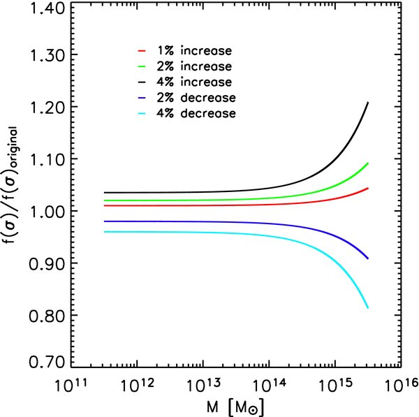
Figure 1. Sensitivity of the mass function to systematic shifts in individual halo masses. Changes are shown relative to a baseline mass function, taken to be the fitting form of Table 4. A small shift of 2% in the halo masses can lead to changes of up to 5%–10% in the high-mass tail of the mass function.
Download figure:
Standard image High-resolution imageThese results, arising from the exponential sensitivity of the mass function at high masses, demonstrate an important point: given the level of uncertainties in halo masses due to numerical errors and the definition of the halo mass itself, it is not possible to derive a mass function prediction from simulations at sub-percent or percent accuracy without a consistent study of how individual halo masses vary as a function of simulation parameters like force resolution, time step size, starting redshift, etc. Fortunately, it is already known that (b = 0.2) FOF halo masses, over the mass range of interest, are relatively robust to changes in simulation parameters; as demonstrated in Heitmann et al. (2005), individual halo masses as computed by six different codes with varying resolutions and time-stepping schemes typically agree to better than 2%. Additionally, Lukić et al. (2007) have provided criteria for running simulations so as to minimize systematic errors from a variety of possibilities. Our task is to ascertain whether error control can be further improved systematically.
We focus here on three main possible systematic errors in the mass function (based on experience from Heitmann et al. (2005) and Lukić et al. (2007)): (1) small systematic errors in individual halo masses due to force resolution, focusing attention on the high-mass tail, (2) the known systematic bias in individual FOF masses as a function of the number of particles in the FOF halo (Warren et al. 2006), and (3) systematic errors from missing long wavelength power due to the necessarily finite box size. We also note the easily avoidable pitfall of using approximate fits for the transfer function rather than the numerical solution (see Appendix A for details). As discussed below, and in more detail in Appendix A, all of these effects can induce systematic errors in the mass function and need to be taken into account. (Figure 2 shows the effect of various corrections.)
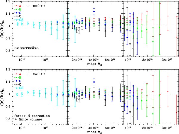
Figure 2. Uncorrected (upper panel) and corrected (lower panel) results for the ratio of the mass function to our best-fit model at z = 0. Most of the difference is due to the correction for the finite particle sampling of the halos. A detailed description of the error bars is given in Appendix A.
Download figure:
Standard image High-resolution imageAll numerical simulations are necessarily run with a finite force resolution, balancing the need for high spatial resolution with suppression of noise/collisional artifacts. Below the chosen force softening length, the forces between the particles asymptote to zero. As a result, the halos that are formed tend to be "puffed out" in a simulation with coarse force resolution. The net effect is that—for heavy halos, with scale radii significantly greater than the softening length—the mass of a given halo in a simulation with coarse resolution tends to be greater compared to a simulation with better resolution. This implies that the halo mass and hence the mass function determined from a simulation study would be higher compared to the "ideal" case of infinite force (and mass) resolution. Although this effect is known to be small (Lukić et al. 2007), it can certainly be significant at the percent level of error in the mass function. We also note that the effect of force resolution depends on the details of how halos are found using the SO and FOF algorithms. Here we focus on the case of FOF halos; a discussion of the impact of force resolution on SO halos is given in Tinker et al. (2008). In Appendix A, we provide a detailed analysis of the errors due to finite force resolution and how to correct for them. In our simulations, we find that finite force resolution effects can be accounted for by introducing a corrected rescaled mass Mc via

Here M is the uncorrected halo mass and is the force resolution measured in kpc of the different runs as specified in Table 2. In our case, the biggest correction applied is ≈0.6% for individual halo masses for the A runs (with a force resolution of 97 kpc). This results in a systematic lowering of approximately 2% in the high-mass tail of the mass function (primarily run A) as shown in Figure A3 in Appendix A.
As stated earlier, we identify halos with a standard FOF algorithm, with a linking length, b = 0.2. Although halos with only a small number of particles (∼20) can be reliably found with the FOF algorithm, accurate mass estimation requires keeping many more particles within individual halos. Aside from simple considerations of particle shot noise, there is an inherent systematic error and scatter in the definition of an FOF halo mass with particle number, even in the absence of all other limitations, as pointed out by Warren et al. (2006). For ideal NFW halos (and for isolated relaxed halos in simulations), this effect was studied by Lukić et al. (2009) and represents the best possible scenario. To avoid problems with too few particles in halos, we restrict attention to halos with at least 400 particles. With this cutoff, the agreement in the mass function for the overlap regions across the various boxes is within a few percent. After first applying the FOF sampling correction suggested by Warren et al. (2006), we find that a slightly modified correction of the form ncorrh = nh(1 − n−0.65h) brings the results from the nested boxes in good agreement, as shown in Appendix A in Figure A4. We stress that this adjustment is purely empirical, targeted at matching halo masses in overlapping boxes. The study in Lukić et al. (2009) shows that for NFW halos, the correction depends on nh as well as on the halo concentration. Thus, in principle, one may expect the FOF sampling correction to be more complex than a simple compensation based on nh; we leave a more detailed analysis for future work. The use of the restriction nh ⩾ 400 appears, however, to make the correction predominantly dependent on nh alone. The net correction in halo mass due to finite force and mass resolution, for our simulation suite, can then be written as

Last, we consider systematic errors due to the finite volume of simulations. There are three sorts of effects of this type. The first is simply that the number of halos at high masses will be poorly sampled, and the mass function in this region will have large statistical error bars due to shot noise (Poisson fluctuations). This is purely a question of having sufficient total simulation volume. The second effect is the fact that missing large-scale modes, with k < 2π/L (L is the box size in linear dimension), lead to a suppression of structure formation, and hence of the mass function, as reduced power is available for transfer from linear to nonlinear scales as evolution proceeds. Mass functions measured from simulations must therefore account for the infrared cutoff in the variance of matter fluctuations σ(M). The extended PS approach has been found to work well in compensating for this effect (see Lukić et al. 2007 and references therein), and we follow it here. For our simulations, this volume correction is relevant only for the small box (GS) set of simulations, where L = 178 Mpc, and affects only the low mass halos. Applying the EPS method to the smallest box shifts the masses by 2%.
The third finite-volume effect is related to the (effective) number of independent realizations, i.e., the sample variance. Because halos are biased tracers of the density field, the mass function in a given, sufficiently large, target volume is sensitive to the local mean density as set by the scale-independent bias. In a large-volume simulation, local sub-volumes will have fluctuating average densities and these will add another component to the mass function variance, aside from shot noise. There are two ways to address this: (1) because of the high covariance between the small number of low k modes in a simulation and its high k modes, run either very large boxes where the relevant low k modes (in terms of power transfer) are sampled sufficiently well, or (2) run a sufficient number of statistically independent large-volume boxes.
In either case, one can successfully estimate the variance using a simple halo model prescription and linear theory for density fluctuations (Hu & Kravtsov 2003); details are given in Appendix A.3. An important point to note is that all simulation boxes necessarily have a definite infrared cutoff set by the box size. This can in fact be tuned to control the mass function variance: smaller boxes have smaller variance because they have less low-frequency power. Of course, one cannot make the box too small because then the mass function will be biased low as in the EPS discussion above.
If one runs only one box, then resampling techniques such as the jackknife may have to be used to estimate the associated errors (see, e.g., Tinker et al. 2008; Crocce et al. 2010). These techniques can be susceptible to misestimation of errors for smaller boxes, due to the assumed independence of subvolumes of the simulation box. To estimate our errors, we prefer to use independent realizations for a given simulation volume. This has the advantage that the individual modes of fluctuations are truly independent across realizations and hence averaging over them represents the true variance for each set of runs. We note that for large boxes ∼2 Gpc, jacknife sampling works well (Tinker et al. 2008). However, since we have 10 independent 2 Gpc box runs (A), we can use the different realizations to estimate the errors. (Additionally, the increased mass resolution in each box makes one less susceptible to the finite sampling problem in determining FOF halo masses.) The sample variance errors were computed by taking the ratio of the variance for each of the runs divided by the number of realizations of each run; details are discussed in Appendix A.3. As stated already, with this method one also has the extra flexibility of tuning the low frequency cutoff to optimize the mass variance (if the only simulation goal is to produce an accurate mass function).
Our results from this section are summarized in Figure 2. The upper panel shows the raw simulation results and the lower panel includes our three corrections for force resolution, finite sampling, and finite volume. In order to show the effects more clearly, we display the ratio of the mass function to our best fit to the data, as derived in the next section. Once the simulation parameters for initial redshift, force resolution, and box size are chosen in a suitable way for studying the mass function, the major correction required is the one due to finite mass resolution.
4. REFERENCE ΛCDM MODEL
4.1. Mass Function at the Present Epoch
After having analyzed possible systematic errors and corrected for them in all our simulations, we now investigate the mass function for the reference ΛCDM cosmology specified in Table 1 (model 0) at z = 0. The effective simulation volume, combining all of our runs, is approximately 250 Gpc3. The simulations provide coverage of halo masses ranging from that relevant for individual bright galaxies all the way to clusters, with good statistics. Although the total volume is dominated by the set of runs with box size of 2778 Mpc, the other runs are very helpful in checking for and investigating systematic errors as seen above, and in extending the simulation reach to lower halo masses.
As previously discussed, a convenient form to express the scaled differential mass function f(σ, z) is (Jenkins et al. 2001)
Here n(M, z) is the number density of halos with mass M, ρb(z) is the background density at redshift z, and σ(M, z) is the variance of the linear matter power spectrum P(k) over a length R,

when smoothed on the scale R(M) = (3M/4πρb)1/3 with the top-hat filter W(x) = 3[sin(x) − xcos(x)]/x3. We write σ(M) ≡ σ for brevity in the following. The redshift dependence is encapsulated in the growth factor D(z) which is normalized in such a way that D(0) = 1. As mentioned earlier, the advantage of this definition of the mass function is that to a reasonable accuracy it does not explicitly depend on redshift, power spectrum, or cosmology; all of these are encapsulated in σ(M, z).
A popular numerical fit for the differential mass function f(σ) is given in Sheth & Tormen (1999, ST hereafter). The expression for the ST mass function is

where A, a, and p are three parameters tuned to simulation results with a = 0.707 (a = 0.75 is proposed as a better estimate in Sheth & Tormen 2002), p = 0.3, and A = 0.3222. The parameter A is fixed by the normalization condition that all dark matter particles reside in halos, i.e.,
We note that, as a practical matter, the lower halo mass cutoff in numerical simulations is too large to test this particular assumption. So, in principle, one could leave this constant as a free variable in the fitting process. With the normalization condition fulfilled, the ST mass function has two free parameters, a and p. δc is the density threshold for spherical collapse. In an Einstein–de Sitter cosmology, δc = 1.686, independent of redshift. For Ωm ≠ 1, the value for δc shows insignificant dependence on cosmology (Lacey & Cole 1993). We checked that including the cosmology dependence in δc does not explain the redshift evolution of f(σ) seen in our simulations. In the following, we therefore keep δc = 1.686 as a fixed value.
In order to obtain a fit for f(σ, z), we need to compare Equation (5) with the binned mass function obtained from the simulations. We measure the number density of halos in a bin of size Δln M with mass limits [M1, M2], as

In the limit that Δln M → 0, we can write Equation (9) as

and hence fdata(Mbin, z) can be written as
where Mbin = ∑Mi/Nbin, and the summation is over all the halos in a bin. When combining all the boxes from the various simulations, we vary Δln M and make it small enough to ensure that Equation (10) holds within the accuracy of the data. The results are shown in Figure 3. We find that four bins per decade equally divided in ln -space between 1011and1014 M☉ and 15 bins per decade between 1014and3 × 1015 M☉ are sufficient for the mass function to converge within the measurement errors for z = 0 and z = 1. This corresponds to a bin size of Δln M = 0.25 between 1011and1014 M☉ and Δln M = 0.06 between 1014and1016 M☉. For z = 2, four bins per decade in mass (Δln M = 0.25) are sufficient for the measurements to converge within the accuracy of the data.

Figure 3. Ratio of the mass function data at z = 0 with respect to our z = 0 fit for different choices of the number of bins. For halos of mass ⩽1014 M☉, four bins per decade in mass are sufficient for the mass function data to converge. For halos of mass ⩾1014 M☉, the result converges for a choice of 15 bins per decade.
Download figure:
Standard image High-resolution imageFigure 4 compares different mass function expressions given previously as compared to our new simulation results at z = 0. The expressions for different fits are given in Table 3. Some of these expressions, derived from earlier simulations, are significantly discrepant—especially at high masses—at the 20% level and higher. Results from more recent simulations are in much better agreement, partly because the cosmology runs are much closer. We note that exact correspondence cannot be expected because the mass function is not universal; we defer a discussion of this point to Section 5.

Figure 4. Ratio of various mass function fits derived in previous studies with respect to the results of this paper at z = 0. The binned numerical data are the points with error bars; the ratios are taken with respect to the analytic fit to the numerical data specified by Equation (12). Because the fits are based on runs with different cosmologies, exact correspondence cannot be expected (since the mass function is not universal).
Download figure:
Standard image High-resolution imageTable 3. Mass Function Fitting Formulae Derived in Previous Studies
| Reference | Fitting Function f(σ) | Mass Range | Redshift Range |
|---|---|---|---|
| Sheth & Tormen (2002) | ![$f_{{\rm ST}}(\sigma)= 0.3222\sqrt{\frac{2(0.75)}{\pi }} \exp \left[- \frac{0.75\delta _c^2}{2\sigma ^2}\right]\left[ 1+ \left(\frac{\sigma ^2}{0.75\delta _c^2} \right)^{0.3} \right]\frac{\delta _c}{\sigma }$](https://content.cld.iop.org/journals/0004-637X/732/2/122/revision1/apj387314ieqn1.gif) |
Unspecified | Unspecified |
| Jenkins et al. (2001) | 0.315exp [ − |ln σ−1 + 0.61|3.8] | −1.2 ⩽ ln σ−1 ⩾ 1.05 | z = 0–5 |
| Warren et al. (2006) | ![$ 0.7234\left(\sigma ^{-1.625} + 0.2538\right)\exp \left[-\frac{1.1982}{\sigma ^2}\right]$](https://content.cld.iop.org/journals/0004-637X/732/2/122/revision1/apj387314ieqn2.gif) |
(1010–1015) h−1 M☉ | z = 0 |
| Reed et al. (2007) | ![$0.3222\sqrt{\frac{2(0.707)}{\pi }}\left[1+ \left(\frac{\sigma ^2}{0.707\delta _c^2} \right)^{0.3} +0.6G_1(\sigma) + 0.4G_2(\sigma)\right]$](https://content.cld.iop.org/journals/0004-637X/732/2/122/revision1/apj387314ieqn3.gif) |
−0.5 ⩽ ln σ−1 ⩾ 1.2 | z = 0–30 |
![$\times \frac{\delta _c}{\sigma }\exp \left[ -\frac{0.764\delta _c^2}{2\sigma ^2}- \frac{0.03}{(n_{{\rm eff}}+3)^2\left(\delta _c/\sigma \right)^{0.6}}\right]$](https://content.cld.iop.org/journals/0004-637X/732/2/122/revision1/apj387314ieqn4.gif) |
|||
| Manera et al. (2010) | ![$f_{{\rm ST}}(\sigma)= 0.3222\sqrt{\frac{2a}{\pi }} \exp \left[- \frac{a\delta _c^2}{2\sigma ^2}\right]\left[ 1+ \left(\frac{\sigma ^2}{a\delta _c^2} \right)^{p} \right]\frac{\delta _c}{\sigma }$](https://content.cld.iop.org/journals/0004-637X/732/2/122/revision1/apj387314ieqn5.gif) |
(3.3 × 10¹³–3.3 × 10¹⁵) h−1 M☉ | z = 0–0.5 |
| Crocce et al. (2010) | ![$A(z)\left[ \sigma ^{-a(z)} + b(z)\right]\exp \left[-\frac{c(z)}{\sigma ^2}\right]$](https://content.cld.iop.org/journals/0004-637X/732/2/122/revision1/apj387314ieqn6.gif) |
(1010–1015) h−1 M☉ | z = 0–1 |
Notes. Various fits from previous studies shown in Figures 4 and 6 for FOF halos of linking length b = 0.2 are listed. For Manera et al. (2010), the parameter values are (a, p) = (0.709, 0.248) at z = 0 and (0.724, 0.241) at z = 0.5. For Crocce et al. (2010), the parameter values are A(z) = 0.58(1 + z)−0.13, a(z) = 1.37(1 + z)−0.15, b(z) = 0.3(1 + z)−0.084, andc(z) = 1.036(1 + z)−0.024. For Reed et al. (2007), ![$G_1(\sigma)= \exp \big[-\frac{(\ln \sigma ^{-1}-0.4)^2}{2(0.6)^2}\big]$](https://content.cld.iop.org/journals/0004-637X/732/2/122/revision1/apj387314ieqn7.gif) and
and ![$G_2(\sigma)= \exp \big[-\frac{(\ln \sigma ^{-1}-0.75)^2}{2(0.2)^2}\big]$](https://content.cld.iop.org/journals/0004-637X/732/2/122/revision1/apj387314ieqn8.gif) .
.
Download table as: ASCIITypeset image
In order to obtain a fitting form to our results, we begin with the ST fit as the starting point, although, as shown in Figure 4, the ST mass function deviates from the simulation results by as much as 40% at the high-mass end. As a first step to improving the accuracy of the ST mass function, we drop the normalization requirement and refit all three parameters A, a, and p to the numerical data. With this approach, the simulation data can be fit to an accuracy of 10%–15%, significantly worse than the statistical errors of our data set (see also Manera et al. 2010). The remaining inadequacy of the ST fit can be addressed in different ways. For example, Warren et al. (2006) introduced a fourth parameter into the ST functional form and refitted the other three parameters to their simulation data, finding a best-fit mass function:

with AW = 0.7234, b = 1.625, c = 0.2538, and d = 1.1982. As shown in Figure 4, this particular fit also severely underestimates the mass function at high masses, by up to ∼30%. While adequate as a fitting form over a finite range, Equation (11) diverges when the normalization condition is imposed (Equation (8)). To avoid this, we present a new fitting function for f(σ). This is the simplest ST modification that does not diverge but adds one extra parameter,  (for
(for  we recover the ST mass function):

We use a χ2 technique to determine the best fit f(σ) that matches the mass function data obtained by combining all of the ΛCDM runs. That is, we minimize
where f(σ)mod, f(σ)data, and Δf(σ)data are given by Equations (12), (10), and (A4), respectively.
Minimizing χ2 gives the best-fit parameter values:  ,
,  ,
,  , and
, and  with a χ2 per degree of freedom of 1.15. The subscript "0" indicates that the best-fit values are specified at z = 0. The results are summarized in Table 4. As mentioned above, this expression does not diverge when the normalization condition is imposed, however, the best fit does not lead to a normalization of unity. As shown in Figure 5, this modified expression agrees with the simulation data to better than 2% accuracy at z = 0. As further discussed in Section 4.2, a simple redshift dependence has to be introduced into the fitting function to obtain agreement at the same accuracy level at higher redshifts.
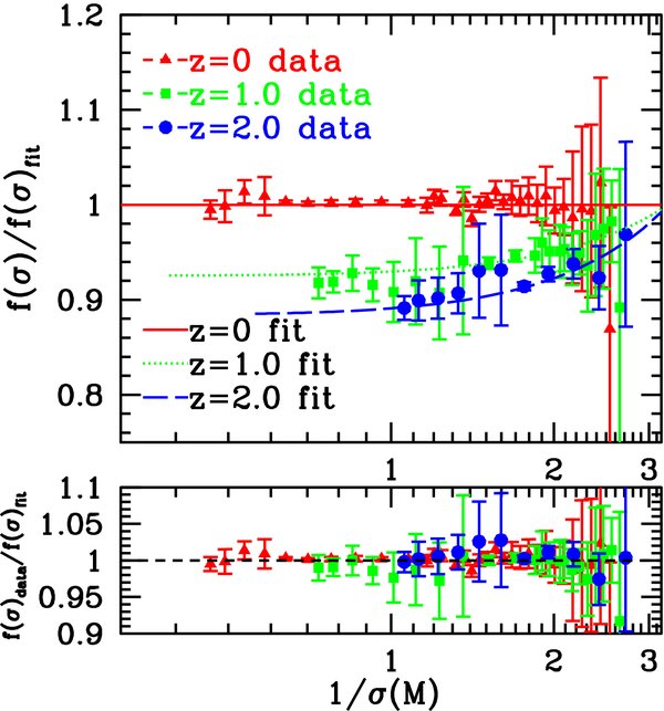
Figure 5. Ratio of the mass function data to the z = 0 fit of Equation (12) (reference flat red line). The z = 1 and z = 2 data sets demonstrate that redshift evolution is important and must be taken into account; the curves show the corresponding fits following the time dependence as parameterized in Equations (14). The lower panel shows the ratio of the measured mass function at the three different redshifts to the corresponding analytic fits.
Download figure:
Standard image High-resolution imageTable 4. Mass Function Fitting Formula for the Reference ΛCDM Model (Mass Range: 6 × 10¹¹ M☉–3 × 10¹⁵ M☉; Redshift Range: z=0–2)
![$f^{\rm mod}(\sigma,z)= \tilde{A}\sqrt{\frac{2}{\pi }} \exp \left[- \frac{\tilde{a}\delta _c^2}{2\sigma ^2}\right]\left[ 1+ \left(\frac{\sigma ^2}{\tilde{a}\delta _c^2} \right)^{\tilde{p}}\right]\left(\frac{\delta _c \sqrt{\tilde{a}}}{\sigma }\right)^{\tilde{q}}$](https://content.cld.iop.org/journals/0004-637X/732/2/122/revision1/apj387314ieqn15.gif) |
|
|---|---|
| Redshift Evolution | |
 |
Download table as: ASCIITypeset image
4.2. Redshift Evolution and Universality
The z = 0 mass function fit of Section 4.1 has a default universal form. However, as remarked previously, it is known that the mass function deviates from universality—as a function of redshift—for ΛCDM cosmologies. Recent results include those of Tinker et al. (2008) who found the SO halo mass function to evolve by 20%–30% from redshift z = 0 to 2.5. As shown in Figure 5, this deviation can be as much as 10% between redshifts z = 0and2 for FOF halos, in agreement with the results of Crocce et al. (2010). In this section, we extend our fitting function to include the redshift evolution of the mass function. We parameterize the possible redshift evolution of each parameter via a simple power-law form
In order to ensure that the expression for the redshift evolution reproduces the mass function at any intermediate redshift when interpolated or even extrapolated, we fit two redshift outputs at a time. Thus, we have three values for each parameter. The final set of parameters is the average of the three values obtained using redshift outputs in pairs. Figure 5 shows that the power law model of Equations (14) is able to capture the redshift evolution with an accuracy of better than 3% within the range of 0.6 ⩽ 1/σ ⩽ 2.4. We find that only two of the four parameters of Equations (14) show any redshift evolution. The best-fit values for the parameters αi describing the redshift evolution are α1 = 0.11, α2 = 0.01, α3 = 0.0, and α4 = 0.0. We note that the non-universal redshift evolution is suppressed at higher redshifts as the effect of the cosmological constant is reduced and matter-domination takes over. To recap, our analytic best fit to the mass function data uses one extra shape parameter compared to ST to match the z = 0 data, and then introduces a simple z dependence (two more parameters) to capture non-universal behavior.
We also explore the option of allowing for a redshift dependence, δc(z), as determined by the spherical collapse model. For the ΛCDM cosmology adopted here, the spherical collapse calculation yields δc = 1.674, 1.684, and 1.686 respectively for z = 0, 1, and 2. As expected, at z = 2, δc approaches the value expected for the Ωm = 1 cosmology. Allowing for this redshift dependence does not mitigate the redshift dependence of the other fitting parameters; including δc(z) changes the value of  to 0.799/(1 + z)0.024 (in fact increasing the redshift dependence) while the other parameters remain unchanged. Therefore, adding δc(z) does not help explain the z dependence seen in our simulations, and we do not include it in our fit.
High-statistics studies of the evolution of the FOF mass function have been carried out previously. In an investigation focusing mainly at high redshifts, to explain the violation of universality, Reed et al. (2007) proposed an effective spectral slope neff set by the halo radius, parameterized as

This new effective slope induces a redshift dependence in the mass function. However, as shown in Figure 6, the analytic fit of Reed et al. (2007) is not in good agreement with our results (see also Bagla et al. 2009 which studies the dependence of the mass function universality on the initial matter power spectrum). This discrepancy indicates that high-redshift evolution of the mass function is slower compared to that at lower redshifts. Crocce et al. (2010) also use a simple power-law form to fit for redshift evolution. Our reference model and the parameters of Crocce et al. (2010) are very close; consequently, their results are significantly closer to ours, except at very high masses, where their fit appears to deviate. Here, discrepancies may result from the use of an approximate transfer function5 and a small systematic offset in their fitting procedure at high masses (cf. their Figure 8). Taking this offset into account we find that the actual numerical results are in agreement at the few percent level. The expressions for the fitting functions of Reed et al. (2007) and Crocce et al. (2010) are given in Table 3. Figure 7 shows the abundance dn/dln M as measured in our simulation along with the analytic fits. Figure 8 summarizes the results from this section, showing the mass function at different redshifts and our best-fit results.
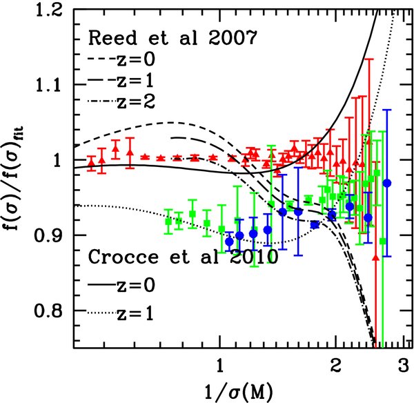
Figure 6. Redshift-dependent mass function fits as introduced by Reed et al. (2007) and Crocce et al. (2010) compared with the numerical data of this work. Aside from disagreement in the overall shape, the results of Reed et al. (2007) underestimate the amount of evolution indicating that high-redshift evolution of the mass function is slower compared to that at lower redshift. The agreement with Crocce et al. (2010) is better (at the 4%–5% level), except for the runaway at high masses (see discussion in Section 4.2).
Download figure:
Standard image High-resolution image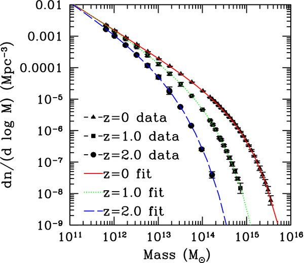
Figure 7. Halo mass function as measured in our simulations at three different redshifts, z = 0, 1, and 2 along with the analytic fit at each redshift.
Download figure:
Standard image High-resolution image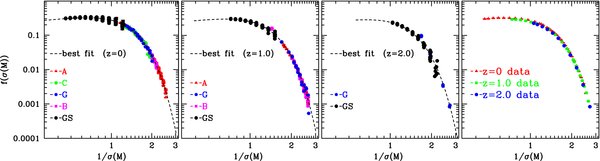
Figure 8. Mass functions for the ΛCDM simulations shown at redshifts z = 0, 1, and 2, for different simulation boxes. The line is the mass function fit. The far right panel shows the mass function obtained by combining all the boxes. Note that the results for the different redshifts do not line up perfectly and therefore a redshift-independent fit cannot be found at very high accuracy.
Download figure:
Standard image High-resolution image4.3. Mass Function-derived Large-scale Halo Bias
The evolution of the spatial distribution of halos has been studied in detail in Cole & Kaiser (1989) and subsequently in Mo & White (1996) and Sheth & Tormen (1999). These studies assume that dark matter halos are biased tracers of the underlying dark matter distribution. The halo bias in general is stochastic and a nonlinear function of the underlying density field (Schulz & White 2006; Seljak & Warren 2004). In addition, it also depends on the assembly history of the halos (Dalal et al. 2008). As discussed in Sheth & Tormen (1999), within the halo model, the large-scale deterministic bias can be derived knowing the shape and evolution of the mass function. It is known that the peak-background split model prediction for the bias using the Sheth–Tormen or Warren et al. (2006) mass function is in disagreement with direct numerical calculations of this quantity obtained from ratios of correlation functions or power spectra in simulations (see, e.g., Lukić 2008; Padmanabhan & White 2009, and Tinker et al. 2010). Given a more accurate mass function, it is easy to check if the halo model approach now produces a better answer for the halo bias. To test this—following Sheth & Tormen (1999) and Cole & Kaiser (1989)—we now obtain the expression for the large-scale bias using our expression for the mass function.
The expression for bias can be written in terms of the conditional and unconditional mass functions as
where N(m, z1|M, V, z0) is the average number of halos of mass m which collapsed at z1 and in a cell of volume V which contains the mass M at z0 and ν = δ2c/σ2.
In the large-scale limit, the "peak-background split" formalism (Sheth & Tormen 1999; Cole & Kaiser 1989) prediction for the halo bias for mass m at redshift z can be derived as follows: define the peak height ν1 relative to the background ν0 as ν210 = (δ1 − δ0)2/(σ21 − σ20). Keeping the leading order terms in the expression gives ν210 = ν21(1–2δ0/δ1). One can then Taylor expand Equation (16) and use Equation (7) to obtain the bias predicted by the ST mass function in Lagrangian space. Converting to bias in Eulerian space, the result is
Similarly, using the mass function fit based on our simulation results, Equation (12), the large-scale bias can be expressed as
Figure 9 shows the predicted bias compared to the ST result. Due to the difference in the two mass function fits, we find a corresponding change in the large-scale bias of 10%–15%. Note that this difference is maximal for halos in the mass range 1013–1014 M☉. Unfortunately, the fact that the (nominally) improved prediction for the bias lies consistently below the ST prediction makes it deviate even further from numerical calculations for the large-scale bias as a function of mass. This behavior is in excellent accord with the analysis in Lukić (2008) performed using the Warren et al. (2006) mass function fit and simulation data from Lukić et al. (2007). Therefore, we conclude that the simple halo model result for the halo bias does not converge correctly as one essential ingredient—the mass function accuracy—is systematically improved. Our conclusion is consistent with other recent studies: Tinker et al. (2010) have found that SO halos are systematically biased 10% higher compared to the Sheth–Tormen bias prediction. Manera et al. (2010) also conclude that a prediction based on a simple peak-background ansatz is inadequate to find agreement with their simulation results.
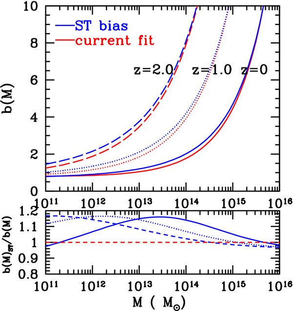
Figure 9. Large-scale halo bias from the peak-background split formalism, derived from the mass function. The upper panel shows the large-scale bias at redshifts z = 0, 1, and 2. The lower panel shows the ratio between the bias derived here and the Sheth–Tormen bias for z = 0, 1, and 2. Note that we assume that the redshift of observation is the same as the redshift of formation of the halos (zform = zobs).
Download figure:
Standard image High-resolution image5. MASS FUNCTION FOR WCDM COSMOLOGIES
Based on our results in Section 4, which include a mass function fit at 2% accuracy for the reference ΛCDM cosmology, we now investigate how well this fit works as cosmological parameters are varied. Including the dark energy equation of state parameter, w, as a phenomenological constant, we consider a suite of wCDM models: 37 simulations that span a wide range of cosmological parameter values. The values of the parameters for each simulation are given in Table 1 with the ranges being specified in Equation (2). Although each simulation is individually large, the volume of each run is much smaller (2.2 Gpc3) than for the combined reference ΛCDM runs (250 Gpc3). Therefore, the statistics of the halos, especially at high masses, is not as well determined in this case. Consequently, we do not attempt an as careful a statistical fit for the mass function for the wCDM models, although we do use all the relevant error controls. For each run we compute the Poisson error and the sample variance error using Equation (A5).
Interestingly, it turns out that the modified universal fit already derived for the ΛCDM case, including the redshift evolution, also works in a relatively unbiased way for the suite of wCDM cosmologies at the 5%–10% level. However, clear systematic violations of universality are observed from this suite of runs as cosmological parameters are varied (Figures 10, 11, and 12). The figures show the ratio of the wCDM mass functions at z = 0, 1, and 2 obtained from our simulation suite with respect to the reference ΛCDM mass function. We find that the FOF mass function shows systematic ∼5%–10% variations (in both directions) with respect to the ΛCDM reference (at higher masses, the statistics is not good enough to make very precise statements), although universality is preserved at the 2%–3% level up to 1/σ ∼ 1.2. Note that for some choices of cosmological parameters the difference is as large as 10% especially at the high-mass end at z = 0.
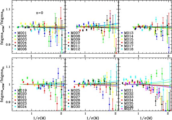
Figure 10. Test of universality of the mass function for wCDM cosmologies (the G runs) at z = 0. The range of the cosmological parameters covered by the simulations is given in Table 1. The ratio is taken with respect to the best-fit mass function for the ΛCDM case at z = 0. The lines show the ratio of the fit if δc is cosmology dependent in the ΛCDM fit.
Download figure:
Standard image High-resolution image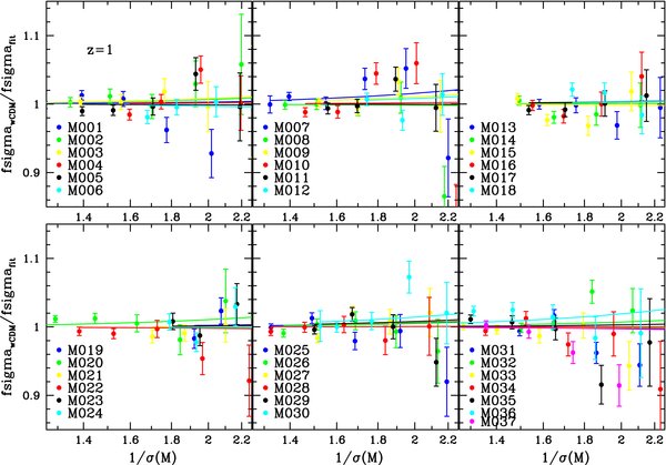
Figure 11. Ratio of the mass function for wCDM cosmologies to the best-fit mass function for the ΛCDM case at z = 1. The lines show the ratio of the fit if δc is cosmology dependent in the ΛCDM fit.
Download figure:
Standard image High-resolution image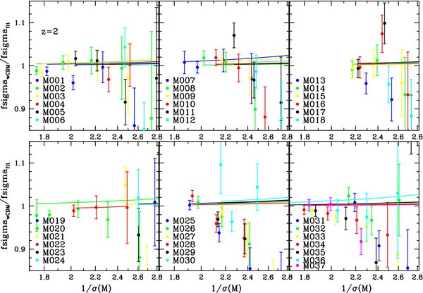
Figure 12. Ratio of the mass function for wCDM cosmologies to the best-fit mass function for the ΛCDM case at z = 2. The lines show the ratio of the fit if δc is cosmology dependent in the ΛCDM fit.
Download figure:
Standard image High-resolution imageWe also investigate the cosmology dependence of δc as predicted by spherical collapse. Details of the calculation of δc as a function of cosmology are given in Appendix B. (See also Pace et al. 2010 for a detailed study.) The lines in Figures 10, 11, and 12 represent the ratio of our fit at a particular redshift when δwCDMc is used in our expression in Table 4 to the reference ΛCDM fit at that redshift. Adding δwCDMc agrees qualitatively with the wCDM runs; however, the difference predicted by the spherical collapse model is too small to be in quantitative agreement with our results. Note that δwCDMc depends only on two parameters for a flat wCDM cosmology, namely Ωm and w. However, universality can also break down as other parameters change, and some of these—σ8, h, and ns—are also varied here. There is currently no theoretical framework to understand the breaking of universality with these parameters. At higher redshift, wCDM cosmologies are expected to converge to the Ωm = 1 cosmology. This is roughly the trend seen in Figures 11 and 12 for the case of z = 1 and z = 2.
Figure 13 summarizes our findings in this section showing the best-fit mass function f(σ) at three redshifts and the simulation results from the 37 cosmologies. Overall, all cosmologies are described reasonably well by our new fit. Points to be noted include: (1) an approximately universal fit describes the wCDM mass function at 10% accuracy over an observationally useful range of cosmological parameters, and (2) universality of the mass function is systematically broken at this level of accuracy within both wCDM (for example, models 22, 25, and 35) and ΛCDM cosmologies (models 31 and 34).

Figure 13. Approximate universality of the wCDM mass functions, all 37 models shown together.
Download figure:
Standard image High-resolution imageGiven the current observational state of the art, a wCDM mass function determined at the 5%–10% level over the range of cosmologies studied here appears adequate for data analysis. However, this is not likely to be the case for the next generation of observations. To extend our work further would require a series of large simulations with their mass function results interpolated along the same lines as already achieved for the power spectrum to scales of order k ∼ 1 h Mpc−1 (Lawrence et al. 2010).
6. DISCUSSION
In this work, we study the mass function of dark matter halos over a wide range of masses (6 × 10¹¹–3 × 10¹⁵ M☉ for a reference ΛCDM model) and a redshift range of z = 0–2 for a large range of wCDM cosmologies. An FOF algorithm with a linking length of b = 0.2 is used for halo identification. The primary aims are to control numerical errors and gain sufficient statistical power for cosmological parameter estimation and testing of the universality of the mass function. For a reference ΛCDM model, we achieve a 2% error in determining the mass function. At this level of numerical control, deviations from universality (in both cosmological parameters and redshift evolution) can be studied systematically. Our level of numerical control is approaching the N-body baseline level—necessary but by no means sufficient—required by next-generation cosmological surveys. The quest for high accuracy in the "N-body" mass function has a natural stopping point at the percent level simply because at this point many other physical processes become important (e.g., baryonic effects; Stanek et al. 2009). Moreover, the connections to observations need to be directly modeled and end up adding their own significant contribution to the overall error.
We use a large number of high-resolution simulations for studying the mass function in a single ΛCDM cosmology. These simulations are used to establish the error control methodology in order to obtain an accurate mass function. Error sources systematically studied here include effects of finite force resolution, FOF particle sampling bias, and systematics induced by finite-volume effects.
Using the more accurate mass function fit for this reference cosmology, we also rederive the large-scale halo bias using the "peak-background split" approach. Compared to previous results obtained with the ST fit, the halo bias changes by 10%–15% between z = 0and2, and is systematically lower. Unfortunately, instead of improving the agreement with direct numerical measurements of halo bias (computed by taking ratios of correlation functions), the use of an improved mass function only increases the discrepancy. This points to an essential difficulty with the halo modeling approach. We will return to this problem elsewhere (Z. Lukić et al. 2011, in preparation).
After studying the mass function in detail for the reference ΛCDM cosmology, we extend the range of cosmological parameters by considering a suite of wCDM simulations. The range of parameters is set by the current constraints on cosmological parameters. The simulation parameters for the runs are given in Tables 1 and 2. We note that the reference mass function fit provides a good description of the wCDM results at an accuracy of ∼10%, however, with systematic deviations that point to clear violations of the universality of the mass function, not only in wCDM parameter space, but also within the set of ΛCDM models (and models very close to ΛCDM).
The breaking of universality as a function of different ΛCDM parameters is studied in Jenkins et al. (2001), Tinker et al. (2008), and Warren et al. (2006). These studies have shown that universality breaks down at the 20% level when σ8 and Ωm are varied. Also Courtin et al. (2011) have studied how universality breaks down for quintessence cosmology and found similar variation of universality with cosmology as reported here. The universality of the mass function in the presence of early dark energy has been studied in Grossi & Springel (2009). We find that universality in the mass function holds at the 10% level as a function of cosmological parameters (the wCDM suite) and redshift (wCDM and the reference ΛCDM model).
Given the breaking of universality discussed here (see also Tinker et al. 2008), it is not clear what the utility of fitting formulae for the mass function might be for observations that actually do require theoretical predictions at the percent level of accuracy. An extensive future simulation campaign will be needed to properly come to grips with this problem. Nevertheless, to provide a compact description of our results, we derive a fitting formula that agrees with our reference ΛCDM simulation results at 2% accuracy over the redshift range of z = 0–2 and the mass range of 6 × 10¹¹–3 × 10¹⁵ M☉. The fitting function is a simple modification of the Sheth–Tormen form with one extra shape parameter to improve the fit at z = 0 and two extra evolution parameters. This form does not lead to divergences if the normalization condition that all mass resides in dark matter halos is imposed. It holds at the 10% level of accuracy for a broad class of wCDM cosmologies with the redshift evolution taken into account.
A special acknowledgment is due to supercomputing time awarded to us under the LANL Institutional Computing initiative. Part of this research was supported by the DOE under contract W-7405-ENG-36 and by a DOE HEP Dark Energy R&D award. S.B., S.H., K.H., Z.L., and C.W. acknowledge support from the LDRD program at Los Alamos National Laboratory. K.H. and Z.L. were supported in part by NASA. M.W. was supported in part by NASA and the DOE. K.H., S.H., and M.W. thank the Aspen Center of Physics where part of this work was completed. S.B. and Z.L. acknowledge useful discussions with Darren Reed. We thank the referee for a careful reading of the manuscript and for a number of useful insights and suggestions.
APPENDIX A: SYSTEMATIC ERRORS IN MASS FUNCTION MEASUREMENTS FROM N-BODY SIMULATIONS
A.1. Initial Conditions
One issue regarding initial conditions not considered in Lukić et al. (2007) is the accuracy of the transfer function used for generating the linear power spectrum. Usually computed via Boltzmann codes such as CMBFAST (Seljak & Zaldarriaga 1996) or the related code CAMB,6 the transfer function is in principle known to 0.1% accuracy (Seljak et al. 2003), which is quite sufficient for the task at hand. Due to their simplicity, however, analytic fits have sometimes been used. As an example, the formula given in Eisenstein & Hu (1999) agrees with numerical results to better than 5% (around a central region of parameter space). However, using such a fit (as for example, in the work of Crocce et al. 2010) gives two errors: (1) an incorrect mapping from σ(M) to M (Figure A1, where using the wrong transfer function yields a noticeable overprediction of the halo abundance at high masses), and (2) a systematic error in the underlying simulation which no longer accurately represents the correct cosmology. It is therefore important to use the most accurate transfer function available to obtain precision results from simulations.

Figure A1. Ratio of halo abundances using the fitting formula given in Table 3 for two different transfer functions—the analytic fitting form of Eisenstein & Hu (1999) and that generated using CAMB. The ratio of the mass function for two different transfer function choices is shown. At the high-mass end, the mass function is overestimated by several percent if the analytic fit is used.
Download figure:
Standard image High-resolution imageA.2. Error Due to Finite Force Resolution
To study the effect of finite force resolution errors quantitatively, we use two simulations with identical initial conditions and cosmological parameters. Both the runs have a box size of length 1.3 Gpc and 10243 particles. One of the simulations is run using GADGET-2 with a force resolution of 50 kpc as specified in Table 2. The other was run with a particle-mesh (PM) code with a 20483 spatial grid, corresponding to a force resolution of approximately 700 kpc. We call the two runs G and PM, respectively.
Since the runs have identical initial conditions, halos in both runs should have approximately the same locations. For each halo in run G, we expect to find a corresponding "match" in run PM. However, as shown in Lukić et al. (2007), for a given force resolution, halos below a certain mass (or equivalently containing a certain number of particles) are not reliably formed. For the PM run, the associated prediction for the minimum number of particles required for a halo to form is ≈400 (see Equation (30) in Lukić et al. 2007). In order to make sure that the mass function is not suppressed due to this effect, the actual number of particles in a halo should be larger than this minimal value. We find that ∼2000 particles per halo is a good choice and hunt for matched halo pairs only above a corresponding mass of 2 × 10¹⁴ M☉ (or halos containing more than 2500 particles). This being the case, we find that nearly 95% of the halos have their centers within ∼400 kpc (consistent with the force resolution of the PM run). The ratio between the matched halo masses averaged over all the matched pairs is shown as a histogram in Figure A2. As a function of mass bin (lower panel), the peak of the ratio distribution remains essentially unchanged, with median values ranging from 1.041 to 1.034. Roughly speaking, the data are therefore consistent with an overestimate by approximately 4% in individual halo masses in the PM run, independent of the mass. (Note that the mean of the ratio distribution has a slightly stronger dependence on halo mass, ranging from 1.06 to 1.036, resulting from tail effects in the distribution.)

Figure A2. Distribution of the ratio of halo masses in the low-resolution (PM) and high-resolution (G) runs in units of 1014 M☉. The top panel shows the distribution for all halos with M ⩾ 1.3 × 10¹⁴ M☉ in run G that have a matching halo in the PM run; more than 95% of the halos have matched pairs within 347 kpc. The bottom panel shows the distributions for different mass bins demonstrating that the shift in the halo mass between the high- and low-resolution runs is practically independent of mass.
Download figure:
Standard image High-resolution imageSince the effect is small, a simple linear extrapolation is sufficient to correct each of the runs in Table 2 in order to predict the halo mass in the limiting case. The corrected mass Mc is given by

Here M is the uncorrected halo mass and is the force resolution measured in kpc of the different runs as specified in Table 2. (We have checked that this formula is consistent with another smaller set of PM simulations—2563 particles, 10243 mesh, with a force resolution of 334 kpc.) The biggest correction needed is ≈0.6% for individual halo masses for the A runs (with a force resolution of 97 kpc). This results in a systematic lowering of approximately 2% in the high-mass tail of the mass function (primarily run A) as shown in Figure A3.
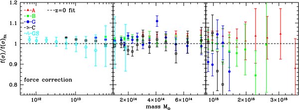
Figure A3. Impact of the correction for finite force resolution errors on the mass function. The ratio of the simulation results with respect to the best-fit z = 0 mass function given in Equation (12) is shown. We display results for different box sizes separately to study possible numerical artifacts in the overlapping regions of different boxes. The effect only alters high-mass halos (for a comparison see the uncorrected mass function in Figure 2) and leads to a systematic lowering of the mass function by 2% at the high-mass end.
Download figure:
Standard image High-resolution imageA.3. Error Due to Finite Number of Particles in a Halo
The reason for the scatter and bias in FOF masses due to the finite number of particles in a halo is that the FOF algorithm aims to capture the mass of a halo within a certain isodensity contour, rendering the halo mass sensitive to the accurate determination of this boundary. Undersampling of the halo will lead to particles on the halo boundary tending to link more to particles close by than in the case of a well-sampled halo with the end result of overestimating the halo mass (see Lukić et al. 2009 for details).
In their work on the mass function, Warren et al. (2006) suggested a correction for the FOF halo mass of the form, ncorrh = nh(1 − n−0.6h), where nh indicates the number of particles in a halo. This adjustment is an empirical finding using a set of nested volume simulations. This correction factor has been used in recent studies, for example, by Tinker et al. (2008) and Crocce et al. (2010). In broad outline this result is consistent with the findings of Lukić et al. (2009). The adjustment formula lowers masses for halos with smaller numbers of particles and depends only on the number of particles within a halo. Unfortunately, this adjustment cannot be applied in all circumstances, as the details of the correction can depend on the details of the individual simulations. Additionally, this adjustment should not be applied at small particle numbers, where it is known to overcompensate.
The problem with FOF halo masses described above is best seen in our simulations by comparing results for the mass function in overlapping mass bins across the different-sized simulation boxes (with differing mass resolutions, see also Warren et al. 2006). This is shown in the upper panel in Figure 2. In our work we combine five different box sizes (multiple runs for each box size) with different mass and force resolution to cover a large range of halo masses. The figure shows the ratio of the raw simulation results from the five different box sizes with respect to our best-fit mass function. In the absence of a systematic bias across the boxes, the results should match up within Poisson errors, but this is clearly not the case.
In order to correct for the finite particle sampling of the halos we investigate different strategies. If all halos are NFW, then following the analysis in Lukić et al. (2009) we can implement a correction which takes into account the concentration and the number of particles in a halo. The general trend is that higher concentration halos should have smaller corrections while, overall, the corrected halo masses would be lower (as in the simulations). Since our force resolution is not sufficient to reliably determine the concentration of the halos, we can use the known mass–concentration relation (including scatter) to estimate a concentration for each halo. It turns out that such a correction lowers the mass function overall by almost 10% but does not provide an accurate match between different boxes. Therefore, this simple modeling fails to explain the quantitative results from the simulations, presumably because the concentration estimates are too crude and because of the irregularities of roughly 20% of the halos.
We therefore use a conservative strategy of a large minimal number of particles per halo, nh > 400, and apply the empirical nh-dependent correction. We find that the suggested form in Warren et al. (2006) can be slightly improved by changing it to

The result of applying the correction according to the above formula is shown in Figure A4.
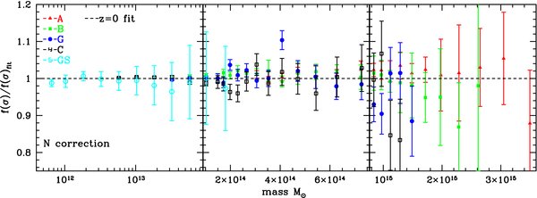
Figure A4. Impact of finite sampling errors on the mass function. The ratio of the simulation results with respect to the best-fit z = 0 mass function given in Equation (12) is shown. The effect from finite sampling is much larger than the effect due to finite force resolution.
Download figure:
Standard image High-resolution imageA.4. Finite Volume Effects
In this appendix, we analyze the third finite-volume effect mentioned in Section 3 in detail, related to the (effective) number of independent realizations, i.e., the sample variance. Because we are using a simple, independent simulation box technique, we compute the variance for each of the runs—separately for each fixed value of the simulation volume—over the number of realizations of each run. Thus, for each run (A, B, C, etc.) we calculate

where Nruns is the number of realizations for a particular fixed-volume run (e.g., Nruns = 10 for the A runs).  is the average number density of halos in a bin averaged over all the realizations and n is the number density for a single realization. Note that this error includes both Poisson fluctuations of halos and the separate sample variance contribution. The fractional error on f(σ) is then calculated as
where we include only Poisson errors and ignore the error in determining Mbin due to Poisson fluctuations.
The fractional errors are shown in Figure A5. The results can be directly compared to simple estimates of the variance using the halo model following Hu & Kravtsov (2003). With this approach, one finds
where V is the volume of the simulation box, Rbox = (3V/(4π))1/3, W(x) is the spherical top-hat window function, and b(M,z) is the large-scale bias from Equation (18). The first term above is the shot noise contribution and the second term gives the sample variance contribution to the total variance. Note that the lower limit of the integral is specified by the simulation box size. For the larger boxes, this is irrelevant, but for the GS runs, the effect is significant, as also shown in Figure A5, which demonstrates good agreement between our results and the theoretical estimate. Note that by using independent smaller volume runs we can reduce the error due to sample variance by a significant amount (of course one should keep in mind that too-small boxes will systematically bias the mass function low, a small and correctable bias in our case, as shown in Figure 2).

Figure A5. Total fractional error (Poisson plus sample variance) for each simulation run. Here, the error bars denote the "error on the errors" which is simply the Poisson error. As an example, for the A runs with 10 realizations, the "error on the errors" is ∼30%. The dotted lines represent the corresponding halo model predictions from Equation (A5) for an infinite volume box, while the solid curves represent the same predictions for the actual simulation sizes used. The two remain close except for the GS runs; see the text for a discussion. For all the runs, there is satisfactory agreement between the theoretical estimates (solid curves) and the actual results from the simulations.
Download figure:
Standard image High-resolution image
APPENDIX B: SPHERICAL COLLAPSE CALCULATION OF δwCDMc
In this appendix, we summarize the calculation of δc for any cosmology as predicted by the spherical collapse model. We are interested in perturbations in a homogeneous sphere. The full nonlinear equation for perturbations (Pace et al. 2010) is
Keeping only the linear terms in Equation (B1) gives

where  is the Hubble factor at a redshift z = 1/a − 1. Assuming we want to calculate the value of δc at z = 0, we require the sphere to collapse at z = 0. We set the initial conditions δ'i = 0. We varied δ'i and checked that the final value of δc is quite insensitive to the value of δ'i. We solve Equation (B1) such that δ becomes a large number at z = 0 (numerically we attain convergence for δ = 108) for a chosen initial perturbation, δi. We iteratively converge to the value of δi such that collapse happens at z = 0, i.e., δ = 108 at z = 0. Once δi is computed by solving Equation (B1), we use that value to solve Equation (B2). The solution of Equation (B2) gives the value of δc at z = 0. Thus, for a given cosmology, i.e., for given values of Ωm and w, solving Equations (B1) and (B2) gives δc at a given redshift, z.
Footnotes
- 5
M. Crocce (2010, private communication).
- 6