THE FIRST GALAXIES: ASSEMBLY OF DISKS AND PROSPECTS FOR DIRECT DETECTION

Andreas H. Pawlik; Miloš Milosavljević; Volker Bromm

doi:10.1088/0004-637X/731/1/54

1. INTRODUCTION

The hierarchical assembly of dark matter halos and the cooling and condensation of the cosmic gas to form stars and galaxies inside them (Rees & Ostriker 1977; Silk 1977; White & Rees 1978; Blumenthal et al. 1984) are major pillars of the current cold dark matter (CDM) paradigm of structure formation in the universe with cosmological constant Λ. Both (semi-) analytical arguments (e.g., Tegmark et al. 1997; Reed et al. 2005; Naoz et al. 2006) and simulations (e.g., Bromm et al. 2002; Abel et al. 2002; Yoshida et al. 2006) suggest that the first stars have formed at redshifts as high as z ∼ 30, when the universe was just about a percent of its present age (for reviews see, e.g., Barkana & Loeb 2001; Bromm & Larson 2004; Bromm et al. 2009). Their light ended the Dark Ages that followed the release of the cosmic microwave background (CMB) radiation at z ≈ 1100 and fundamentally transformed the universe during a landmark period called the epoch of reionization (for reviews see, e.g., Loeb & Barkana 2001; Ciardi & Ferrara 2005; Barkana & Loeb 2007; Trac & Gnedin 2009; Stiavelli 2009; Loeb 2010).

Future observations with telescopes such as, for example, Planck,¹ the Low Frequency Array,² the Murchison Widefield Array,³ the Atacama Large Millimeter Array,⁴ and the James Webb Space Telescope (JWST)⁵ will test our current theoretical understanding of the formation of stars and galaxies at these early times. A fascinating prospect is the detection of line and continuum radiation from the first galaxies with JWST. The ratio of the hydrogen and helium Balmer line luminosities from recombining gas has been proposed as a telltale signature that distinguishes between first-generation, metal-free (Population III) and subsequent metal-enriched (Population II) star formation or between stellar sources and black holes (e.g., Tumlinson & Shull 2000; Bromm et al. 2001; Oh et al. 2001; Tumlinson et al. 2001; Schaerer 2002, 2003; Johnson et al. 2009). In addition, the detection of Lyα, molecular, or metal line cooling radiation from high redshifts would probe the gravitational assembly of the gas in the first halos (e.g., Haiman et al. 2000; Dijkstra 2009, Mizusawa et al. 2005; Appleton et al. 2009), offering direct insights in the structure and dynamics of the first galaxies and the surrounding intergalactic medium (e.g., Santos 2004; Dijkstra et al. 2006, 2007; Verhamme et al. 2006; Laursen et al. 2011).

The combination of upcoming observations with JWST and other future telescopes with detailed numerical supercomputer simulations of the first galaxies and reionization will transform our knowledge of structure formation in the universe. Most of the numerical effort in early galaxy formation has concentrated on investigating the properties of the very first building blocks of galaxy assembly, minihalos, and dwarf galaxies with virial temperatures ≲10⁴ K, corresponding to halo masses ≲10⁸ M_☉ at z ≳ 10 (e.g., Abel et al. 2002; Bromm et al. 2002; Wise et al. 2008; Turk et al. 2009; Stacy et al. 2010; Greif et al. 2010). A key result emerging from the existing work is that the luminosities of these very low mass objects are, unless magnified by gravitational lensing, too low, by at least one order of magnitude, to be detected in even very deep exposures with JWST (Greif et al. 2009; Johnson et al. 2009; see also, e.g., Loeb & Haiman 1997; Haiman & Loeb 1998; Oh 1999; Oh et al. 2001; Trenti et al. 2009). The light collected in future deep-field observations with the JWST may thus be dominated by emission from dwarf galaxies inside halos that are about 10 times more massive, M_vir ∼ 10⁹ M_☉.

Our goal is to extend and complement existing numerical work on the first galaxies by investigating the role played by galaxies inside halos with masses M_vir ≳ 10⁹ M_☉, at times before and during the epoch of reionization, when these galaxies were assembling, possibly contributing a significant fraction (if not most; e.g., Loeb 2009; Wise & Cen 2009; Salvaterra et al. 2010; Raičević et al. 2011) of the ionizing emissivity in the universe, to the present day, when these galaxies may be found in the Local Group as fossil probes of the beginnings of galaxy formation (for reviews see, e.g., Mateo 1998; Tolstoy et al. 2009; Ricotti 2010; Mayer 2010). Indeed, the new field of "dwarf archaeology" may hold the key to unravel the interplay of star and galaxy formation at the end of the cosmic dark ages (Frebel & Bromm 2010). Here, we report our first steps toward achieving this goal by studying the assembly of dwarf galaxies in halos reaching virial masses M_vir ∼ 10⁹ M_☉ at z = 10 using cosmological smoothed particle hydrodynamics (SPH) simulations.

We utilize a zoomed simulation technique that allows us to simulate the gravitational and hydrodynamical processes of dwarf galaxy formation at high resolution while keeping information about structure formation at large representative scales. Our simulations include radiative cooling from atoms and molecules in gas of primordial composition but ignore star formation and the associated feedback. We post-process our simulations with idealized models for star formation and employ population synthesis models to estimate the prospects for a direct detection of the first galaxies with the upcoming JWST. Other aspects of the simulated galaxies, such as, e.g., their role as reionization sources, will be investigated in subsequent works, in which we will explicitly account for the effects of star formation and associated feedback.

The structure of this paper is as follows. In Section 2, we describe the setup of our simulations. Then, in Section 3, we present our results, and subsequently discuss the assembly of the simulated halo, its structure, and dynamics at redshift z = 10 and the properties of the disks it hosts. In Section 4, we combine our simulations with assumptions about star formation to assess the observability of the first galaxies in future observations with JWST. In Sections 5 and 6 we discuss, respectively, implications and limitations of our work. Finally, in Section 7, we summarize our work.

Throughout this work we assume ΛCDM cosmological parameters Ω_m = 0.258, Ω_b = 0.0441, Ω_Λ = 0.742, σ₈ = 0.796, n_s = 0.963, and h = 0.719, which are consistent with the 5 year (Komatsu et al. 2009) and 7 year (Komatsu et al. 2011) analyses of the observations with the Wilkinson Microwave Anisotropy Probe satellite. Distances are expressed in physical (i.e., not comoving) units, unless noted otherwise.

2. SIMULATIONS

We use a modified version of the N-body/TreePM SPH code gadget (Springel 2005; Springel et al. 2001b) to perform a suite of high-resolution zoomed cosmological hydrodynamical simulations in a box of size L = 3.125 h⁻¹ Mpc comoving. The box size was chosen after inspection of published dark matter halo mass functions (e.g., Reed et al. 2007) such that the box contains at least one halo of mass ∼10⁹ M_☉ at redshift z = 10.

We carry out SPH simulations of primordial metal-free gas including non-equilibrium radiative cooling from both molecular and atomic species and from atomic species only. In the following, these two types of simulations will be distinguished by an additional NOMOL at the end of the label of the atomic cooling simulation. The simulations are performed with the gravitational forces softened over a sphere of Plummer-equivalent radius epsilon . Our simulations Z4 and Z4NOMOL, which are obtained by zooming into a parent cosmological simulation four times, use a force softening radius epsilon = 0.1 h⁻¹ kpc comoving applied to all particles.

We employ the entropy-conserving formulation of SPH (Springel & Hernquist 2002) with N_neigh = 48 neighbor particles per SPH kernel. We limit the radius h of the SPH kernel to above a fraction f_h of the softening length, h ⩾ f_h epsilon , where f_h = 0.01. The simulations are summarized in Table 1.

Table 1. Simulation Parameters

Simulation	m_gas^a	m_DM^b	Comoving ^c	Cooling
Z4	4.84 × 10²	2.35 × 10³	0.1	Molecular
Z4NOMOL	4.84 × 10²	2.35 × 10³	0.1	Atomic

Notes. ^aGas particle mass in the refinement region (M_☉). ^bDark matter particle mass in the refinement region (M_☉). ^cGravitational softening radius (h⁻¹ kpccomoving).

Download table as: ASCII Typeset image

2.1. Initial Conditions

All simulations start at redshift z = 127. Initial particle positions and velocities are obtained by applying the Zel'dovich approximation (Zel'dovich 1970) to particles arranged on a Cartesian grid. We adopt a transfer function for matter perturbations generated with cmbfast (version 4.1; Seljak & Zaldarriaga 1996).

To achieve high resolution we make use of the zoomed simulation technique (Navarro & White 1994; we use the same code as in Greif et al. 2008). We first perform a simulation in which the initial conditions are set up using 2 × 64³ (dark matter and gas) particles arranged on a uniform Cartesian grid. We then use the friends-of-friends (FOF) halo finder, with linking parameter b = 0.2, built into the substructure finder subfind (Springel et al. 2001a) to locate an FOF halo with mass ≳10⁹ M_☉ at z = 10 in this simulation. Using subfind, we determine the most bound particle of this FOF halo and let it mark the center of the region that we wish to resimulate. We compute the associated virial radius r_vir by determining the radius of the sphere around the most bound particle within which the average matter density equals 200 times the critical density at z = 10. The particles within a region of radius r ≲ 3r_vir around the most bound particle are traced back to their locations in the initial grid where they mark the region of refinement.

Subsequently, all parent particles in a cube enclosing the refinement region are replaced by $8^{N_{\rm l}}$ daughter particles, where N_l is the zoom level. Our simulations Z4 and Z4NOMOL employ N_l = 4 and hence in these simulations the daughter gas (dark matter) particles have masses m_g = 484 M_☉ (m_DM = 2350 M_☉). To reduce numerical artifacts due to the large difference in the particle masses for particles inside and outside the refinement region (mass ratios $8^{N_{\rm l}}$ ), the refinement region is surrounded by N_l − 1 concentric, nested layers in which the parent particles are successively replaced by $8^{N_{\rm l} - 1}$ , $8^{N_{\rm l}-2}$ , ..., 8 daughter particles and, hence, the particle masses vary gradually, by discrete factors of 8, with increasing distance to the refinement region. The simulation is then re-run after applying the Zel'dovich approximation to evolve all particles to the starting redshift z = 127.

2.2. Chemistry and Cooling

All our simulations include radiative cooling in the optically thin limit. We assume that the gas is of primordial composition using a hydrogen mass fraction X = 0.752 and a helium mass fraction Y = 1 − X. We follow the non-equilibrium chemistry and cooling of H₂, D, HD, D⁺, H⁺, H, D, and He, and we include H⁻ and H⁺₂ assuming their equilibrium abundances (Johnson & Bromm 2006; Greif et al. 2010).

In simulation Z4, gas cools by collisional ionization and excitation, the emission of free–free and recombination radiation, Compton cooling off the CMB, and emission of radiation by molecular hydrogen and hydrogen deuteride (HD). If initial abundances are expressed as number density with respect to hydrogen, where n_H = Xρ_g/m_H with ρ_g being the gas density at z = 127, and m_H is the mass of the proton, we choose: H₂ = 1.1 × 10⁻⁶, D = 2.6 × 10⁻⁵, HD = 10⁻⁹, D⁺ = 1.2 × 10⁻⁸, H⁺ = 3 × 10⁻⁴, He⁺ = 0, and He⁺⁺ = 0, from which the initial abundances of the remaining species (H, D, He) as well as the abundance of electrons are obtained through application of conservation laws. Our choices for the initial abundances are consistent with computations of cosmological abundances in the early universe (e.g., Lepp & Shull 1984; Galli & Palla 1998).

Thanks to molecular cooling, gas in simulation Z4 may reach temperatures as low as ∼10² K. Simulation Z4NOMOL is identical to simulation Z4 except that the formation of molecular hydrogen is suppressed, as would be the case in the presence of a strong photodissociating Lyman–Werner radiation background (Stecher & Williams 1967; Haiman et al. 1997). Gas in simulation Z4NOMOL therefore cools only via atomic processes, which are inefficient in reducing the thermal energy of primordial gas with temperatures below ∼10⁴ K.

2.3. Jeans Floor

Simulations with mass resolutions insufficient to resolve the Jeans mass M_J ≡ (4π/3)ρ_m(λ_J/2)³ by at least N_res ≡ 2 SPH kernel masses M_K ≡ N_neighm_g may suffer from artificial fragmentation (Bate & Burkert 1997). Here, ρ_m is the total (dark matter and gas) mass density, λ_J ≡ c_sπ^1/2(Gρ_m)^−1/2 the Jeans length, c_s = [γk_BT/(μm_H)]^1/2 the adiabatic speed of sound, γ is the ratio of specific heats, and μ is the mean gas particle mass in units of the proton mass. Our finite mass resolution implies a maximum density

$\begin{equation} n_{\rm H, max} = 8 \times 10^5 \, \mbox{cm}^{-3}f_{\rm g} \left(\frac{\gamma }{\mu }\right)^{3} \left(\frac{T}{ 10^4\, \mbox{K}}\right)^3 \end{equation} \tag{ 1 }$

up to which we satisfy the Bate & Burkert (1997) criterion, where f_g ≡ ρ_g/ρ_m.

To satisfy the Bate & Burkert (1997) criterion independent of density we make use of a density-dependent temperature floor (Robertson & Kravtsov 2008; see also, e.g., Schaye & Dalla Vecchia 2008 for a related approach). At each time step and for all gas particles we compute the Jeans mass M_J and compare it to the resolution mass N_resM_K. If the Jeans mass becomes smaller than the resolution mass, then we increase the particle internal energy and, hence, the particle temperature such that the Jeans mass becomes equal to the resolution mass.

3. RESULTS

In this section, we describe the outcome of our simulations. We start in Section 3.1 by briefly presenting the growth histories of the simulated halos. We focus our subsequent discussion on the halo properties at z = 10. In Section 3.2, we discuss the structure of the halos, in Section 3.3 we describe the dynamics of the gas inside them, and in Section 3.4 we investigate the emergence of nested gas disks at the halo centers. Throughout we will discuss differences and similarities between simulation Z4 and simulation Z4NOMOL in which molecular hydrogen formation is suppressed.

3.1. Growth

We use FOF to locate the simulated halos at the final simulation redshift z = 10, and then compute the halo properties as follows. Given an FOF halo, we use subfind to identify its most bound particle and let it mark the halo center. We then compute the virial radius of the halo by determining the radius of the spherical volume centered on the most bound particle within which the average matter density is equal to 200 times the critical density at z = 10. The total mass inside this volume defines the halo virial mass.

We find that r_vir ≈ 3.1 kpc and M_vir ≈ 1.3 × 10⁹ M_☉, independent of the inclusion of molecular cooling. For the adopted cosmological parameters, this virial mass corresponds to ≈3σ fluctuations in the linear theory density field (e.g., Barkana & Loeb 2001). The circular velocity v_c ≡ (GM_vir/r_vir)^1/2 and virial temperature T_vir ≡ μm_Hv²_vir/(3k_B) implied by the virial mass and the virial radius are v_c ≈ 40 km s⁻¹ and T_vir ≈ 42, 000 K, where we have assumed μ = 0.6 appropriate for ionized gas with primordial composition.

After having located the halo at z = 10, we trace its history to higher redshifts using the FOF halo finder together with subfind, as follows. Knowing the FOF halo, the descendant, at redshift z_i corresponding to simulation snapshot i, we locate the FOF halo at redshift z_{i − 1} > z_i corresponding to snapshot i − 1 that shares, among all FOF halos present at z_{i − 1}, the most mass with the descendant. We then use subfind to identify the most bound particle within this FOF halo and obtain the properties of the halo at z_{i − 1} by computing its virial radius and mass in a sphere of average matter density 200 times the critical density at z_{i − 1} centered on the most bound particle.

Figure 1 shows the evolution of the halo mass M_vir (top panel) and its corresponding rate of growth dM_vir/dt (bottom panel) in simulation Z4. The mass growth is described well by an exponential fit M_vir(z) = M₀exp(−αz) (Wechsler et al. 2002) with M₀ = 2 × 10¹¹ M_☉ and α = 0.5. The derived growth rates are consistent with analytical estimates of the rate of growth of the main progenitor (Lacey & Cole 1993). The dot-dashed curve shows the growth rate as given in Equation (A15) of Neistein et al. (2006) with q = 2.3.

3.2. Structure

The left panel of Figure 2 shows density profiles spherically averaged around the most bound halo particle obtained from simulation Z4 at z = 10. The dark matter density profile (red dash-dotted curve; obtained by summing particle masses inside spherical shells and dividing by the shell volume) follows an isothermal shape ρ ∝ r⁻² for radii epsilon ≲ r ≲ r_vir. The gas density profile does not follow the shape of the dark matter profile but shows significant small-scale structure. We have computed the gas density profile both by averaging the SPH particle densities inside spherical shells (green dotted curve) and by summing particle masses inside spherical shells and dividing by the shell volume (blue dashed curve). The two methods for computing the density profile yield different results because the spatial distribution of the gas mass is highly non-uniform, as will be discussed below. We also show the gas density profile in simulation Z4NOMOL (black dotted curve). The dark matter density profile obtained in simulation Z4NOMOL is nearly identical to that from simulation Z4 and hence is not shown.

epsilon — **Figure 2.** Mass and density profiles centered on the most bound halo particle in simulation Z4. In all panels, the vertical lines on the left mark the gravitational softening radius and the vertical lines on the right mark the virial radius at z = 10, the final simulation redshift. Left panel: dark matter (red dash-dotted curve) and gas density profiles at z = 10. The gas densities were computed both by dividing the gas mass summed in shells by the shell volumes (blue dashed curve; this was also done for the dark matter density profiles) and by averaging the SPH particle densities inside shells (green dotted curve). For comparison, the corresponding SPH particle density profile from simulation *Z4NOMOL* is also shown (black dotted curve). The dark matter profile is approximately singular-isothermal for all distances larger than the softening radius. The two steepenings in the gas density profiles at r ≈ 0.07 kpc and r ≈ 0.3 kpc are due to the presence of two nested disks. Middle panel: enclosed gas, dark matter, and total masses at z = 10. Right panel: evolution of the enclosed gas mass. There is a rapid inflow of mass into the central unresolved region r ≲ at 11.5 ≲ z ≲ 12.5.
Download figure:
Standard image High-resolution image

The middle panel of Figure 2 shows the enclosed mass as a function of distance r from the halo center for simulation Z4. The cumulative mass of dark matter dominates the significantly more centrally concentrated cumulative mass of gas for radii r ≳ 0.4 kpc. The buildup of the final gas mass profile shown in the middle panel is illustrated in the right panel of Figure 2. There is a large rapid increase in the mass of the central region (r ≲ epsilon ) around redshift z ≈ 12. In little more than 40 Myr (11.5 ≲ z ≲ 12.5), the central gas mass grows from ∼2 × 10⁷ M_☉ to ∼5 × 10⁷ M_☉. In Section 4, we will assume that this rapid collapse of large gas masses triggers a massive burst of star formation in the central core. The cumulative mass profiles from simulation Z4NOMOL exhibit a nearly identical behavior and again are not shown.

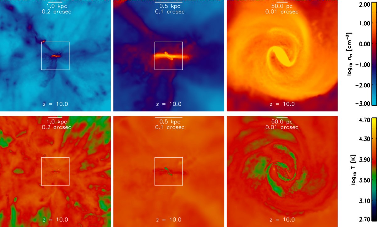
Figures 3 and 4 give further impressions of the baryonic structure of the simulated halos at the final simulation time, i.e., at redshift z = 10. All quantities are shown for both simulation Z4 (Figure 3) and simulation Z4NOMOL in which molecular hydrogen formation was suppressed (Figure 4). The panels in the left columns of Figures 3 and 4 show the hydrogen number densities and temperatures, mapped to a three-dimensional grid using standard mass-conserving SPH interpolation and mass-weighted averaging along the line of sight, within a cubical volume encompassing the virial region.

**Figure 3.** Densities (top) and temperatures (bottom) at z = 10 in simulation Z4 in cubical slices centered on the most bound halo particle. The left panels present edge-on views of the disks and encompass a volume slightly larger than the virial region with radius r_vir ≈ 3.1 kpc. The middle panels are zooms into the cubical regions marked in the left panels. The right panels are zooms into the cubical region marked in the middle panels and are reoriented such that the outer disk is seen face-on. The temperature of the underresolved gas is artificially elevated because of the use of a density-dependent temperature floor to prevent artificial fragmentation. The spirals do not show signs of fragmentation; the gas clump seen in the bottom of the face-on view of the disk (right panels) is a gas-rich subhalo in projection.
Download figure:
Standard image High-resolution image

**Figure 4.** Same as Figure 3, but for simulation *Z4NOMOL*. As in Figure 3, the left-hand and middle panels present edge-on views of the galaxy, and the right-hand panels show the galaxy face-on. Because of the lack of efficient low-temperature coolants and in contrast to simulation Z4 (Figure 3), the gas inside the filaments is at about the same temperatures as the diffuse gas in between the filaments. The temperature of the underresolved gas core is artificially elevated because of the use of a density-dependent temperature floor to prevent artificial fragmentation.
Download figure:
Standard image High-resolution image

The panels show that independent of the inclusion of molecular cooling, gas is organized in four geometrically distinct components: diffuse low-density (n_H ≲ 10⁻² cm⁻³) gas, collimated streams, or filaments, of smooth dense (n_H ≲ 10⁻¹ cm⁻³) gas that penetrate deep into the virialized region, dense (n_H ≳ 10⁻¹ cm⁻³) gas-rich clumps with mostly spherical appearance, and a central dense (n_H ≳ 10¹ cm⁻³) gaseous flattened object seen edge-on. The dense clumps inside the virial radius are associated with low-mass (≲10⁷ M_☉) halos that entered the virial region before z = 10. In the following we refer to these halos as subhalos.

The panels in the middle columns of Figures 3 and 4 are zooms into the cubical regions marked by the white solid rectangles in the panels of the left columns. The panels in the right columns are zooms into the cubical region marked in the panels of the middle columns, but with their coordinate axes rotated. The zooms resolve the central flattened object into two nested disks whose orientations are tilted with respect to each other. The disks cause the steepenings of the gas density profile at r ≈ 0.07 kpc and r ≈ 0.3 kpc seen in the left panel of Figure 2. We let these radii define the sizes of the disks. Note that the disks surround a central unresolved core of radius r ≲ epsilon . The disks will be discussed in more detail in Section 3.4.

The images of the gas temperatures reveal a qualitative difference between simulation Z4 and simulation Z4NOMOL in which molecular hydrogen formation was suppressed. While in both simulations the tenuous gas in between the filaments is at temperatures close to the virial temperature of the halo, the temperatures of the gas inside filaments, subhalos, and the disks are up to an order-of-magnitude lower in Z4 than in Z4NOMOL. Figure 5 shows the molecular hydrogen fraction $\eta _{\rm H_2} \equiv n_{\rm H_2} / n_{\rm H}$ inside the same cubical region as shown in the left panels of Figure 3. The molecular fraction is greatly increased up to $\eta _{\rm H_2} \sim 10^{-3}$ in gas with densities n_H ≳ 1 cm⁻³ and temperatures T ≲ 1000 K, which resides mostly in the filaments and subhalos and in the central halo region.

**Figure 5.** Molecular hydrogen fraction $\eta _{\rm H_2} = n_{\rm H_2} / n_{\rm H}$ at z = 10 in simulation Z4. The image shows the same cubical region as the left panels in Figure 3. The dashed circle marks the virial radius r_vir ≈ 3.1 kpc. The gas inside filaments and subhalos has large molecular fractions $\eta _{\rm H_2} \sim 10^{-3.5}\; {\rm to }\; 10^{-3}$ which enables efficient low-temperature radiative cooling.
Download figure:
Standard image High-resolution image

**Figure 5.** Molecular hydrogen fraction $\eta _{\rm H_2} = n_{\rm H_2} / n_{\rm H}$ at z = 10 in simulation Z4. The image shows the same cubical region as the left panels in Figure 3. The dashed circle marks the virial radius r_vir ≈ 3.1 kpc. The gas inside filaments and subhalos has large molecular fractions $\eta _{\rm H_2} \sim 10^{-3.5}\; {\rm to }\; 10^{-3}$ which enables efficient low-temperature radiative cooling.
Download figure:
Standard image High-resolution image

Without sufficient molecular hydrogen, the intra-halo gas cannot cool efficiently below temperatures T ∼ 10⁴ K as atomic cooling is exponentially suppressed because of the lack of thermal excitation of bound electrons. Gas that is shock-heated to T ≳ 10⁴ K upon entry in the halo then remains hot at T ≈ 10⁴ K until it is incorporated into the dense disks where it cools to slightly lower temperatures. In the presence of a sufficient amount of molecular hydrogen, on the other hand, radiative cooling counters virial heating in the dense gas inside filaments down to temperatures T ≲ 10³ K. The accretion along the filaments then occurs in a cold mode (Wise & Abel 2007; Greif et al. 2008; see also Birnboim & Dekel 2003; Kereš et al. 2005; Brooks et al. 2009; van de Voort et al. 2010 for cold accretion of gas inside more massive halos).

3.3. Dynamics

Figure 6 shows spherically averaged (mass-weighted) profiles of the gas radial velocities v_g,r (left panel) and fractional radial velocities v_g,r/v_g (right panel) at z = 10 in simulation Z4, where v_g = |v_g| and v_g is the gas velocity. For comparison, the corresponding velocities for the dark matter are also shown. The velocities were corrected for the bulk halo motion by subtracting the velocity of the center of mass of all gas particles within the virial region and were calculated relative to the location of the most bound particle. Figure 6 shows that both the dark matter and the gas approach the virial region along mostly radial orbits with similar infall velocities consistent with the halo circular velocity (Section 3.2). Inside it, their velocity distributions, however, differ significantly.

The dark matter isotropizes just upon entry in the virial region, i.e., at r ≈ r_vir (vertical line on the right), which is reflected in a sharp drop of the ratio of radial to total velocity to 3^−1/2 expected for an isotropic velocity distribution (horizontal dotted line in the middle panel of Figure 6). The gas, being able to radiatively cool and lose gravitational energy, keeps streaming with radial velocities that increase toward the halo center and reach maximum values −v_g,r ≲ 60 kms⁻¹. The gas eventually hits the central disk at r ≈ 0.3 kpc where it circularizes. The right panel in Figure 6 shows that at redshift z = 10, in both simulation Z4 and simulation Z4NOMOL, the spherically integrated gas accretion rates are, on average, −r²∫ρ_gv_g,rdΩ ≈ 1 M_☉ yr⁻¹, independent of radius r ≳ 0.07 kpc. The prominent spikes exhibited by the gas accretion rates are due to the infall of gas-rich subhalos along the radial filaments.

The complexity of the gas dynamics within the virial region in simulation Z4 is revealed by the radial and line-of-sight (i.e., along the axis of projection) velocities that are shown, respectively, in the top and bottom panels of Figure 7. The velocity structure of the gas in simulation Z4NOMOL is very similar. The images show views that correspond in size and orientation to the views shown in Figure 3. This allows us to identify structures in the velocity images with those in the images of density and temperature. The velocity images were obtained by mapping particle radial and line-of-sight velocities to a three-dimensional grid using standard SPH interpolation and performing a mass-weighted average along the line of sight to project the grid into a two-dimensional plane.

The line-of-sight velocities (bottom panels in Figure 7) show the kinematic signatures of two rotating disks that are centered on a spatially unresolved core. The inner disk continues to grow in mass not only through accretion of gas from outside the disk plane but also through accretion of gas from within the outer disk to which it is kinematically connected (bottom middle panel in Figure 7). The radial velocity (top panels in Figure 7) shows a complex inflow pattern. The gas stream that points to the top right corner in the top middle panel of Figure 7 is gas ejected by the passage of a gas-rich subhalo from beneath the disk immediately before z = 10. A majority of subhalos appears to be associated with filaments, which resembles the picture of anisotropic accretion of satellites in simulations of massive galaxies and clusters at low redshift (e.g., Libeskind et al. 2011; Knebe et al. 2004).

3.4. The Disks

Figure 8 shows the assembly of the inner and the outer disk in simulation Z4. The disk assembly times and histories in simulation Z4NOMOL are very similar. The inner disk forms at z ≈ 13.5 as a result of a major merger. Initially, it is relatively thin and extended and also shows marked spiral structure. Its gas, however, collapses into the highly concentrated disk that is seen at z = 10 in Figure 3 rather quickly, within a redshift interval Δz ≲ 1, corresponding to ≲40 Myr. The outer disk is assembled from the halo gas at z ≈ 11.5, i.e., ≲100 Myr after the assembly of the inner disk. It grows in size and develops increasingly pronounced spiral structure. In none of our simulations do the disks show signs of fragmentation.

The right panels in Figures 3 and 4 present face-on views of the disks at z = 10. In simulation Z4, the outer disk shows much more developed spiral structure. When seen edge-on (middle panels of Figures 3 and 4), the outer disk in Z4 looks somewhat thinner and more perturbed than the outer disk in Z4NOMOL. The latter may be explained in part by the fact that in simulation Z4, thanks to the efficient low-temperature molecular cooling, subhalos have larger gas fractions than in simulation Z4NOMOL, which increases the chance for possibly violent subhalo–disk interactions.

In simulation Z4NOMOL, the disk gas reaches minimum temperatures T ≳ 8000 K slightly below the temperatures in the diffuse gas and filaments because the increased densities in the disks imply shorter cooling times. In simulation Z4, on the other hand, the disk gas can cool to temperatures T ≲ 1000 K, thanks to the presence of molecular hydrogen. Note that the disk temperatures in simulation Z4 are also determined by the temperature floor enforced to prevent artificial fragmentation (Section 2.3). The temperature floor affects the evolution of the gas for densities above n_H ≳ 10 cm⁻³ in simulation Z4 and densities above n_H ≳ 10⁶ cm⁻³ in simulation Z4NOMOL (see Equation (1)). These densities correspond, respectively, to radii r ≲ 0.3 kpc and r ≲ 0.03 kpc (see Figure 2).

The final mass distributions in the disk region in the simulations Z4 and Z4NOMOL are very similar. In both simulations, the volume inside r ⩽ 0.3 kpc contains gas and total masses of ≈1.4 × 10⁸ M_☉ and ≈2.5 × 10⁸ M_☉, respectively (see Figure 2). These masses amount to ≈65% of the gas mass and to ≈25% of the total mass inside the virial region. In simulation Z4, roughly 20% (35%) of the total (gas) mass within r ⩽ 0.3 kpc is in the central unresolved core, about 30% (40%) is in the inner disks, and about 50% (25%) is in the outer disks. In simulation Z4NOMOL, roughly ≲17% (≲28%) of the total (gas) mass out to radii r ⩽ 0.3 kpc is in the central unresolved core, ≲32% (≲40%) is in the inner disk, and about 51% (≲32%) is in the outer disk.

Figure 9 shows several azimuthally averaged properties of the disks at z = 10 in simulation Z4 and Z4NOMOL. The left panel of Figure 9 shows rotational gas velocities v_g,rot (black curves), adiabatic sound speeds c_s = [γk_BT/(μm_H)]^1/2 (blue curves), and radial velocities v_g,r (red curves), all with respect to the Keplerian velocities v_K = [GM(<r)/r]^1/2 and for both simulation Z4 (solid curves) and simulation Z4NOMOL (dashed curves). The rotational velocities were computed using v_g,rot = (v²_g − v²_g,r)^1/2. For computing the sound speed we have assumed a ratio of specific heats of γ = 5/3 appropriate for a mostly atomic gas and assumed that the cold disk gas is mostly neutral, i.e., μ = 1.2. Both the inner and the outer disks exhibit a high degree of rotational support with the outer disk showing nearly Keplerian motion. The rotational velocities are larger than the sound velocities by factors of ≲5–10. Radial velocities are small compared to rotational velocities at all disk radii and drop sharply to zero once the gas hits the central core at r ≲ epsilon .

The middle panel of Figure 9 shows the gas surface density profiles. In both Z4 and Z4NOMOL, the inner disk, which is resolved with ≳5 gravitational softening radii, is characterized by an exponential surface density profile with scale length 0.015 kpc that extends over several scale lengths. In Z4NOMOL, the outer disk follows an exponential profile over several scale lengths of 0.05 kpc. In Z4, the surface density profile shows significant deviations from an exponential profile. The nearly exponential density profiles of the outer disks in our simulations are only gradually built up and at higher redshifts the density profile in simulation Z4 shows pronounced ripples due to the presence of thick spiral structure.

The right panel of Figure 9 shows the Toomre parameter Q = c_sκ/(πGΣ), where c_s is the velocity dispersion, κ = (4Ω² + rdΩ²/dr)^1/2 is the epicyclic frequency, and Ω = v_g,rot/r is the angular velocity (Toomre 1964). A standard linear theory instability analysis (Toomre 1964; Goldreich & Lynden-Bell 1965; Binney & Tremaine 2008) shows that a gas disk becomes unstable to axisymmetric perturbations if Q ≲ 1; the precise threshold for instability depends on the disk thickness. The linear analysis is confirmed with detailed simulations of disk instability, which also show that a similar criterion applies to the discussion of non-axisymmetric perturbations (see, e.g., the review by Durisen et al. 2007). In computing Q we identify the velocity dispersion c_s with the adiabatic sound speed and we set κ = v_K/r appropriate for Keplerian motion. Both in simulation Z4 and in simulation Z4NOMOL the Toomre parameter Q ≳ 1 for all radii epsilon ≲ r < 0.3 kpc that cover the two disks. In both simulations the inner disk is characterized by Q ≲ 2 while the outer disk is characterized by Q ≳ 2.

The measured Toomre Q parameters imply that the disks in simulation Z4 are somewhat less stable than the disks in simulation Z4NOMOL. This is consistent with the observation that spiral arms in Z4 are more distinct than in Z4NOMOL (right panels in Figures 3 and 4) and is likely a direct consequence of the fact that in simulation Z4 the disk temperatures are significantly lower than in simulation Z4NOMOL thanks to efficient low-temperature cooling by molecular hydrogen. Note that the stability of the outer and of the inner disk in simulation Z4 and the stability of the inner disk in simulation Z4NOMOL may be artificially increased due to the imposed Jeans floor as mentioned above. Note also that in equating the velocity dispersion with the sound speed, we may have underestimated the true velocity dispersion and hence the stability of the disks.

4. DETECTING THE FIRST GALAXIES WITH JWST

One of the main science goals of the upcoming JWST is the detection of light from the first galaxies (Gardner et al. 2006). Here, we present an estimate of the expected flux from the first galaxies based on our simulations of galaxies with halo masses M_vir ∼ 10⁹ M_☉ at z ≳ 10 and investigate their detectability with the instruments aboard JWST.

JWST will observe the first galaxies using deep field imaging and spectroscopy with the Near Infrared Camera (NIRCam) and the Mid Infrared Instrument (MIRI) and using spectroscopy with the Near Infrared Spectrograph (NIRSpec) and also MIRI (for an overview of these instruments see http://www.stsci.edu/jwst; see also Gardner et al. 2006). NIRCam will allow imaging and low resolution (R ≡ λ/Δλ ≲ 100) spectroscopy within a field of view of 2 farcm 2 × 4 farcm 4 and an angular resolution of ∼0 farcs 03–0 farcs 06 in the range of observed wavelengths λ_o = 0.6–5 μm. The multi-object spectrograph NIRSpec will enable medium resolution (R ∼ 100–3000) spectroscopy of up to ∼100 objects simultaneously within a field of view of 3 farcm 4 × 3 farcm 4. NIRSpec will operate in the same wavelength range as NIRCam but at lower angular resolution (∼0 farcs 1). Finally, MIRI will complement NIRCam and NIRSpec by providing imaging, low and medium resolution spectroscopy within the range of observed wavelengths λ_o = 5–28.8 μm and fields of view and angular resolutions of, respectively, ∼2' × 2' and ∼0 farcs 1–0 farcs 6.

4.1. Intrinsic Luminosities

Our estimates of the observability of the first galaxies are based on our simulations of galaxies in halos with masses ∼10⁹ M_☉ at z ≳ 10. We examine and compare two idealized scenarios for star formation derived from the gas accretion rates observed in our simulations, chosen to bracket the range of likely scenarios and parameterized such as to enable the straightforward rescaling and extrapolation of our results. We combine assumptions about the nature of the forming stellar populations with population synthesis models to estimate the luminosities in the Lyα, Hα, and He ii (restframe wavelength λ_e = 1640 Å; hereafter He1640) nebular recombination lines and the intensities of the non-ionizing (combined stellar and nebular) UV continuum (rest-frame wavelength λ_e = 1500 Å; hereafter UV1500). We translate line luminosities and UV continuum intensities into observed fluxes and compare them with the expected flux limits for observations with JWST. Based on extrapolation of our results to galaxies with both lower and larger halo masses, we estimate the number of high-redshift halos that JWST will detect.

The first of the two star formation scenarios explored here assumes that stars form in a single central instantaneous burst with total stellar mass

$\begin{equation} M_\star = 10^6 \, {M}_{\odot }\left(\frac{f_{\star }}{ 0.1}\right) \left(\frac{f_{\rm cool}}{0.01}\right) \left(\frac{M_{\rm vir}}{ 10^9 \, {M}_{\odot }}\right), \end{equation} \tag{ 2 }$

where f_cool is a conversion factor that determines the amount of gas mass available for starbursts inside halos with virial masses M_vir and f_⋆ is the star formation efficiency, i.e., the fraction of the available gas mass that is turned into stars. Setting f_cool = 0.01, this scenario is motivated by the rapid accretion of large gas masses (M_g ≳ 10⁷ M_☉) onto the central unresolved core observed in our simulations of halos with virial masses M_vir ∼ 10⁹ M_☉ at around z ≲ 12 (see the right panel of Figure 2). We choose a relatively high star formation efficiency, f_⋆ = 0.1, expected for the initial bursts (e.g., Wise & Cen 2009; Johnson et al. 2009). The adopted conversion factor f_cool = 0.01 between the gas mass available for star formation and the halo virial mass is consistent with gas collapse fractions in previous simulations of the first galaxies (e.g., Wise et al. 2008; Regan & Haehnelt 2009a).

The second scenario for star formation considered here assumes that stars form continuously at a rate

$\begin{equation} \dot{M}_\star (z) = 0.05 \, {M}_{\odot }\, \mbox{yr}^{-1}\left(\frac{f_\star }{0.05}\right)\left(\frac{\dot{M}_{\rm g}(z)}{ 1 \, {M}_{\odot }\, \mbox{yr}^{-1}}\right) \end{equation} \tag{ 3 }$

in proportion to the rate $\dot{M}_{\rm g}$ at which gas is accreted. Indeed, galaxies with masses ≳10⁹ M_☉ may be sufficiently massive to sustain a moderate level of near-continuous star formation despite ongoing feedback (e.g., Wise & Cen 2009; we discuss the effects of feedback in more detail in Section 6 below). We adopt a gas accretion rate $\dot{M}_{\rm g} \sim 1\, {M}_{\odot }\, \mbox{yr}^{-1}$ that describes the rate of accretion of gas onto the central region with radius r ≲ 0.1r_vir for z ≲ 15 in our simulations of halos with virial masses ∼10⁹ M_☉ (see the right panel of Figure 6). At this radius the gas surface density is roughly in agreement with the critical surface density ≳10–100 M_☉ pc⁻² for star formation in the low-redshift universe (see the middle panel of Figure 9); this critical surface density is further discussed in Section 5 below. We approximately include the effects of feedback from star formation by employing a lower star formation efficiency f_⋆ = 0.05 than used for the starburst. The implied star formation rates $\dot{M}_\star (z) = 0.05 \, {M}_{\odot }\, \mbox{yr}^{-1}$ are consistent with star formation rates found in recent feedback simulations of galaxies inside halos with masses ∼10⁹ M_☉ (e.g., Wise & Cen 2009; Razoumov & Sommer-Larsen 2010).

To compute the luminosities of the stellar populations that form in the two scenarios we must specify the metallicities of the stars, the stellar ages, and the distribution of stellar masses at the time of formation, i.e., the initial mass function (IMF). We first assume that starbursts occur in metal-free gas and form clusters of zero-metallicity stars. We adopt a top-heavy IMF, i.e., an IMF biased toward massive (M_⋆ ∼ 100 M_☉) stars. Such an IMF is expected to characterize the first, metal-free generation of stars which form by radiative cooling from collisionally excited molecular hydrogen (e.g., the review by Bromm et al. 2009).

The IMF of metal-free stars, however, is still subject to large theoretical uncertainty. Stars forming out of gas with an elevated electron fraction, such as produced behind structure formation or supernova (SN) shocks or as inside and near ionized regions, could have characteristic masses substantially less than ∼100 M_☉. This is because the increased electron abundance boosts the production of HD which enables gas to cool to much lower temperatures than is possible with molecular hydrogen alone (e.g., Nakamura & Umemura 2002; Nagakura & Omukai 2005; Johnson & Bromm 2006; Stacy & Bromm 2007; see also Shapiro & Kang 1987 and Clark et al. 2011). We therefore repeat our analysis assuming the formation of metal-free stars with a normal IMF, similar to the one used to describe star formation in the nearby universe.

Enrichment to critical metallicities as low as Z_c ≲ 10⁻⁶to 10^−3.5 Z_☉, where we set Z_☉ ≡ 0.02, will also imply the transition from a top-heavy IMF to a normal IMF (e.g., Bromm et al. 2001; Bromm & Loeb 2003; Schneider et al. 2006; Smith et al. 2009). We therefore complement our study of metal-free starbursts with the study of a burst of stars with above-critical but low metallicities Z ≳ 3 × 10⁻⁴ Z_☉ and normal IMF. Note that a few massive star SN explosions may already be sufficient to enrich the first galaxies to metallicities Z ≳ Z_c (e.g., Scannapieco et al. 2003; Tornatore et al. 2007; Wise & Abel 2008; Karlsson et al. 2008; Greif et al. 2010; Maio et al. 2010). We therefore always adopt above-critical (but low) metallicities Z ≳ 3 × 10⁻⁴ Z_☉ and a normal IMF in the continuous star formation scenario.

We compute the stellar ionizing luminosities expected for the two star formation scenarios using the population synthesis models for zero-age instantaneous bursts and continuous star formation from Schaerer (2003, some of these models have been previously published in Schaerer 2002). The Schaerer (2003) models assume a power-law IMF p(m_⋆) ∝ m^−α_⋆ with Salpeter (1955) exponent α = 2.35 but allow for different ranges for the masses m_⋆ of individual stars. We use the Schaerer (2003) zero-metallicity models for instantaneous starbursts with initial masses in the range 50–500 M_☉ and 1–100 M_☉ to describe metal-free stars with a top-heavy and normal IMF, respectively. We describe the populations of low-metallicity stars using the Schaerer (2003) models with initial masses in the range 1–100 M_☉ and metallicities⁶ Z = 5 × 10⁻⁴ Z_☉. Following Schaerer (2003), we use case B recombination theory (e.g., Osterbrock 1989) to relate the ionizing luminosities of the stellar populations of specific age, mass, and metallicity to the nebular luminosities of the surrounding gas, assuming that all ionizing photons are absorbed, i.e., that the fraction of ionizing photons escaping the galaxy, f_esc, is zero.⁷ We will discuss these assumptions at the end of this section.

Figure 10 shows the luminosities of the Hα and Lyα (left panel) and He1640 (middle panel) nebular lines and the intensities of the non-ionizing stellar and nebular UV1500 continuum (right panel) expected for the two star formation scenarios described above. Note that the luminosities in the Lyα line are related to those in the Hα line by the simple scaling L(Lyα) ≈ 8.6L(Hα) (Tables 1 and 4 in Schaerer 2003). For low metallicity and normal IMF, the starburst scenario implies line luminosities and continuum intensities that are roughly twice as large as those implied by the continuous star formation scenario.

At fixed IMF, the luminosities in Hα and Lyα and the UV1500 continuum intensities of the starbursts are insensitive to the stellar metallicity. The zero-metallicity starburst models with top-heavy IMF imply Hα and Lyα line luminosities and UV1500 continuum intensities larger by about one order of magnitude than those implied by the zero-metallicity starburst model with a normal IMF. In contrast, the starburst luminosities in the He1640 line depend strongly on both the IMF and the stellar metallicity. At fixed normal IMF, a change from low to zero stellar metallicity implies an increase in the He1640 line luminosity by about three orders of magnitude. This is because the exceptionally hot atmospheres of zero-metallicity stars turn them into strong emitters of He ii ionizing radiation (e.g., Tumlinson & Shull 2000; Bromm et al. 2001; Schaerer 2003). An additional change from normal to top-heavy IMF increases the luminosity in the He1640 line by another order of magnitude.

The large differences in He1640 line luminosities offer the prospect of distinguishing observationally between stellar populations made of metal-free and metal-enriched stars and of constraining their IMFs (e.g., Tumlinson & Shull 2000; Bromm et al. 2001; Oh et al. 2001; Johnson et al. 2009). The He1640 recombination line will also be excited due to the emission of ionizing radiation from a central accreting black hole, if present (e.g., Oh et al. 2001; Tumlinson et al. 2001; Johnson et al. 2011). Observationally, accreting black holes could be distinguished from metal-free stellar populations through the detection of their X-ray emission (e.g., Haiman & Loeb 1999). Note though that an evolved stellar population may also contribute to the X-ray emissivity (e.g., Oh 2001; Power et al. 2009). X-ray sources may ionize the gas in a larger region than stellar sources, implying a spatially more extended emission of recombination radiation.

4.2. Observed Fluxes

We translate the line luminosities and UV continuum intensities into observed fluxes to investigate the detectability with JWST. The flux density from a spatially unresolved object emitted in a spectrally unresolved line with rest-frame wavelength λ_e and line luminosity L is given by (e.g., Oh 1999; Johnson et al. 2009)

$\begin{eqnarray} f_\nu (\lambda _{\rm o}) &=& \frac{L \lambda _{\rm e} (1+z) R}{4 \pi c d_{\rm L}^2(z)} \\ &\sim & 3 \,\mbox{nJy}\left(\frac{L}{10^{40} \, \mbox{erg}\, \mbox{s}^{-1}}\right) \nonumber \\ &&\times \left(\frac{\lambda _{\rm e}}{1216 \, {\rm \AA}}\right) \left(\frac{R}{1000}\right)\left(\frac{1+z}{11}\right)^{-1},\qquad\nonumber \end{eqnarray} \tag{ 4 }$

where λ_e is the rest-frame wavelength, λ_o = (1 + z)λ_e the observed wavelength, and d_L ∼ 100[(1 + z)/10] Gpc is the luminosity distance. The UV continuum intensity L_ν of a spatially unresolved object implies an observed flux density (e.g., Oh 1999; Bromm et al. 2001)

$\begin{eqnarray} f_\nu (\lambda _{\rm o}) &=& \frac{L_{\nu }(\lambda _{\rm e})}{4 \pi d_{\rm L}^2(z)} (1+z) \\ &\sim & 1\, \mbox{nJy}\left(\frac{L_{\nu }(\lambda _{\rm e})}{10^{27}\, \mbox{erg}\, \mbox{s}^{-1}\, \mbox{Hz}^{-1}}\right) \left(\frac{1+z}{11}\right)^{-1}.\qquad\nonumber \end{eqnarray} \tag{ 5 }$

Flux densities, f_ν, are related to AB magnitudes, m_AB, via (Oke 1974; Oke & Gunn 1983)

$\begin{equation} m_{\rm AB} = -2.5 \log _{\rm 10} \left(\frac{f_\nu}{\mbox{nJy}} \right) + 31.4. \end{equation} \tag{ 6 }$

The assumption that the lines are spectrally unresolved is excellent for both Hα and He1640, whose line widths Δλ/λ ≲ 10⁻⁴(T/10⁴ K)^1/2 are set by thermal Doppler broadening at temperature T ≲ 10⁴ K (e.g., Oh 1999). We also note that at redshifts z ≳ 10 a transverse physical scale Δl corresponds to an observed angle Δθ = Δl/d_A ∼ 0 farcs 1(Δl/0.5 kpc)[(1 + z)/10], where d_A = (1 + z)⁻²d_L is the angular diameter distance. Hence, if most of the nebular emission originates from within the vicinity of the stellar populations, which we assumed to be concentrated in the halo centers, i.e., at r ≲ 0.1r_vir, the assumption that the emitting regions are spatially unresolved is good for both the Hα and the He1640 line and it applies equally well to the UV continuum.

In contrast, the Lyα line radiation undergoes resonant scattering. Hence, it will likely be additionally spectrally broadened (e.g., Neufeld 1990), and spatially extended with typical angular size Δθ ∼ 15'' (Loeb & Rybicki 1999). It will be damped due to absorption by intergalactic neutral hydrogen (e.g., Miralda-Escude 1998; Santos 2004). Note that Lyα radiation from galaxies at redshifts z ≳ 10 may be particularly strongly damped because the reionization of the universe was probably only accomplished at much lower redshifts (e.g., Fan et al. 2006). On the other hand, scattering off outflowing interstellar gas may help the Lyα radiation to escape (e.g., Dijkstra & Wyithe 2010), and galaxies may reside in an ionized bubble sufficiently large for Lyα photons to redshift away in the expanding universe (e.g., Cen & Haiman 2000; Haiman 2002; Loeb et al. 2005; Wyithe & Loeb 2005; Lehnert et al. 2010). Since we do not treat radiative transfer effects here, Lyα line fluxes implied by Equation (4) must be considered upper limits. In the following we therefore mostly discuss the observability of the Hα and He1640 lines and of the UV1500 continuum.

The He1640 recombination line (λ_e = 1640 Å), as well as the Lyα line (λ_e = 1216 Å) not further discussed here, will be detected by JWST with NIRSpec at a spectral resolution R ∼ 1000, while the Hα line (λ_e = 6563 Å) will be detected with MIRI at a spectral resolution R ∼ 3000. JWST will detect the UV1500 (λ_e = 1500 Å) continuum using NIRCam. As an illustration, Figure 11 shows the minimum stellar mass required for the Schaerer (2003) model starbursts employed here to be observable with JWST. We assume exposures with signal-to-noise ratio S/N = 10 and duration t_exp = 10⁶ s and the currently expected flux limits⁸ for observations with JWST (Table 10 in Gardner et al. 2006; see Panagia 2005 for a graphical presentation and Johnson et al. 2009 for a useful summary). Figure 11 demonstrates that even for exposure times as long as 10⁶ s, JWST will not have sufficient sensitivity to detect stellar populations with masses below ∼10⁵–10⁶ M_☉. JWST will thus not be able to see stellar light from individual first stars (e.g., Oh 1999; Oh et al. 2001; Gardner et al. 2006).

**Figure 11.** Stellar masses M_⋆,min of the lowest mass starburst observable through the detection of the Hα line (solid curves) or the He1640 line (dashed curves) or the UV1500 continuum (dash-dotted curves) with *JWST*, assuming an exposure of t_exp = 10⁶ s and S/N = 10. The masses scale with t^−1/2_exp. Stellar masses derived from the Schaerer (2003) zero-metallicity starbursts with normal IMF, the zero-metallicity starbursts with top-heavy IMF, and the low-metallicity starburst are shown, respectively, in blue, red, and black. The right axis shows the masses M_min = 10³M_⋆,min of halos expected to host a starburst with stellar mass M_⋆,min. The conversion between stellar and halo masses is based on Equation (2) with f_cool = 0.01 and f_⋆ = 0.1. For reference, the dotted curve shows the virial mass (with corresponding labels on the right axis) for a halo with virial temperature T_vir = 10⁴ K. The black dashed curve is not shown because it exceeds the plot range.
Download figure:
Standard image High-resolution image

**Figure 13.** *JWST* starburst counts. Left panel: number of halos N(>z) with redshifts >z and masses >M_min, where M_min is the lowest mass halo capable of hosting a starburst observable through the detection of the Hα line (solid curves) or the He1640 line (dashed curves) or the UV1500 continuum (dash-dotted curves) with *JWST* (Figure 11, right axis). We have assumed an exposure of t_exp = 10⁶ s and S/N = 10. Counts for the model starbursts of zero metallicity and normal IMF, zero-metallicity and top-heavy IMF, and low non-zero metallicity are shown, respectively, in blue, red, and black. The black dashed curve is not shown because it falls below the plot range. Right panel: number of halos N(>f) above z > 10 with observed fluxes >f. The vertical lines show the *JWST* flux limits f_lim ∝ t^−1/2_exp for observations of the Hα line (solid), the He1640 line (dashed) and the UV1500 continuum (dot-dashed), assuming exposures t_exp = 10⁶ s and S/N = 10. The black dashed curve is not shown because it falls below the plot range. *JWST* may detect a few tens (for non-zero metallicities and normal IMFs) up to a thousand (for zero metallicity and top-heavy IMFs) starbursts with redshifts z > 10 in its field of view of ∼10 arcmin². Our estimates for the number counts scale linearly with the assumed starburst durations of τ_sb = 3 Myr and 30 Myr for, respectively, the starbursts with top-heavy and normal IMFs.
Download figure:
Standard image High-resolution image

Figure 12 shows the Hα (left panel) and He1640 (middle panel) recombination line fluxes and the non-ionizing UV1500 continuum fluxes (right panel) for the models presented in Figure 10. The JWST flux limits for exposure times t_exp = 10⁴, 10⁵, and 10⁶ s are indicated by the dotted lines in each panel. The figure reveals that the scenario of continuous star formation implies line and continuum fluxes too low to be observable, even when assuming exposure times as large as 10⁶ s. JWST, however, may see starbursts similar to those modeled here. In exposures with duration ∼10⁶ s, MIRI will detect such starbursts in Hα for all metallicities and IMFs explored.

Figure 12 also reveals that JWST has the potential to constrain the properties of starbursts in galaxies with halo masses as low as ∼10⁹ M_☉, based on the detection of the He1640 line. Indeed, only the zero-metallicity starburst with a top-heavy IMF and observed with an exposure of ≲10⁶ s is detected in He1640. Starbursts inside ≳10–100 times more massive halos would be detected in the He1640 line independent of whether their IMFs are top-heavy. Their nature could then be further constrained by measuring the ratio of the Hα and He1640 line strengths.

Note, finally, that if scattering by the intergalactic gas can be ignored, the total (i.e., integrated over the line) flux in the unresolved Lyα line would be a factor ≈8.6 larger than the total flux in the unresolved Hα line, based on the relation L(Lyα) ≈ 8.6L(Hα) noted above and shown in Figure 10. For a galaxy at redshift z ≈ 10, JWST's NIRSpec is a factor of ≈3 more sensitive to the detection of the redshifted Lyα line than MIRI is to the detection of the redshifted Hα line.⁹ That is, unless radiative transfer effects cause JWST to see less than 1/(8.6 × 3) ≈ 4% of the Lyα line flux, the Lyα line will be easier to detect than the Hα line. Hence, despite the large uncertainties arising from its resonant nature, the Lyα line remains a powerful probe of high-redshift galaxy formation (Partridge & Peebles 1967).

4.3. JWST Number Counts

How many star-forming galaxies can we expect JWST to detect? For simplicity and brevity of the presentation we ignore that galaxies may form stars in a continuous mode and assume that starbursts shine at constant luminosity over a time interval τ_sb. The number of galaxies, per unit solid angle, above redshift z that JWST will detect is then obtained using

$\begin{equation} \frac{dN}{d \Omega }(>z) = \int _z^\infty dz^{\prime }\ \frac{{\it dV}}{dz^{\prime }d\Omega } \frac{\tau _{\rm sb}}{t_{\rm H}(z^{\prime })}\int _{M_{\rm min} (z^{\prime })}^\infty {\it dM}\ \frac{dn(M, z^{\prime })}{{\it dM}}, \end{equation} \tag{ 7 }$

where t_H(z) is the age of the universe at redshift z, dV = cH⁻¹(z)d²_L(1 + z)⁻² is the comoving volume element, H(z) = H₀[Ω_m(1 + z)³ + Ω_Λ]^1/2, and H₀ = 100 h kms⁻¹ Mpc⁻¹ is the Hubble constant. We approximate the comoving number density n(M, z) of halos with mass M at redshift z by the Press–Schechter halo abundance (Press & Schechter 1974; Bond et al. 1991; see, e.g., Zentner 2007 for a recent review). We set M_min(z) = f⁻¹_coolf⁻¹_⋆M_⋆,min(z), where M_⋆,min(z) is the smallest stellar mass observable at redshift z (Figure 11), and we use f_cool = 0.01 and f_⋆ = 0.1 (see Equation (2)).

Figure 13 shows our estimates of the number of observable starbursts in exposures of t_exp = 10⁶ s and S/N = 10. The estimates scale linearly with the assumed durations τ_sb of the starbursts. We set τ_sb = 3 Myr for the zero-metallicity starbursts with top-heavy IMF, which approximately corresponds to the time it takes for its massive ∼100 M_☉ stars to age and explode, upon which further star formation, if not suppressed by SN feedback, will more likely occur inside metal-enriched gas, hence ceasing the zero-metallicity burst. We set τ_sb = 30 Myr for the zero-metallicity and low-metallicity starbursts with normal IMF. Our choice for this longer duration reflects the longer time it takes, on average, for massive stars forming inside bursts with normal IMFs to evolve and explode in SNe. Starburst durations up to ∼30 Myr are consistent with the gas dynamics and the amount of gas available for star formation in our simulations (see Section 3.2 and Figure 2).

Figure 13 demonstrates that JWST will enable the detection of a few tens up to a thousand star-bursting galaxies with redshifts z ≳ 10 in its field of view of ∼10 arcmin². JWST will allow to constrain the predominant nature of the first starbursts as the He1640 recombination line is only detected in significant numbers for the case of zero-metallicity starbursts with top-heavy IMF. Intriguingly, our estimates imply that the first galaxies may be more readily detectable in Hα spectroscopic searches than in UV continuum surveys (see also Figure 12). The expected number of star-bursting galaxies with redshifts z > 10 to be detected with JWST in exposures other than 10⁶ s can be read from the right panel in Figure 13. Our estimates are consistent with previous estimates of JWST starburst counts for similar assumptions about the conversion between stellar and halo mass (e.g., Haiman & Loeb 1998; Oh 1999).

The estimates of the observability of the first galaxies are uncertain due to the assumptions underlying the computation of UV line and continuum emission. We followed Schaerer (2003) and computed the nebular contribution to the stellar luminosities of the first galaxies using Case B recombination theory. Raiter et al. (2010) point out that the Case B approximation ignores photoionizations from excited states and hence underestimates the photoionization rate. At low nebular metallicities and for hot stellar sources, their detailed photoionization models imply Lyα line luminosities and nebular UV continuum intensities larger by factors of 2–3 (see their Figure 10) than expected under the Case B assumption. Raiter et al. (2010) also find that the line luminosities in Hα are insensitive to whether Case B is assumed. Hence, Lyα line and UV continuum emission may provide relatively stronger signatures of star formation inside the first galaxies than suggested here.

Finally, we have assumed that a negligible fraction f_esc of stellar ionizing photons escapes the star-forming regions without being converted into recombination radiation by the surrounding gas, i.e., f_esc = 0. Recent numerical work has emphasized that the escape fraction may depend strongly on the structural properties of galaxies as determined by their masses and internal processes like star formation and feedback (e.g., Fujita et al. 2003; Gnedin et al. 2008; Wise & Cen 2009; Johnson et al. 2009; Razoumov & Sommer-Larsen 2010; Yajima et al. 2010). While escape fractions of order unity f_esc ∼ 0.5 are possible for low-mass (≲10⁹ M_☉) halos with turbulent gas dynamics and amorphous morphology, significantly smaller escape fractions are expected for galaxies that form most of their stars inside dense rotationally supported disks (e.g., Gnedin et al. 2008; Wise & Cen 2009; Razoumov & Sommer-Larsen 2010). The luminosities implied by our assumption of a zero escape fraction can be rescaled to account for non-zero escape fractions by multiplication with the factor (1 − f_esc).

5. DISCUSSION

An interesting outcome of our simulations is the collapse of the halo gas into two extended rotationally supported disks. When and how the first galaxy-scale disks were formed is currently not well understood. Extended disks are found in large-scale hydrodynamical cosmological simulations and in cosmological simulations of individual massive (≳10¹⁰ M_☉) halos or halos at low redshifts (e.g., Kaufmann et al. 2007; Mashchenko et al. 2008; Levine et al. 2008; Sawala et al. 2010; Governato et al. 2010; Schaye et al. 2010; Sales et al. 2010). Cosmological simulations of the first minihalos and low-mass (≲10⁸ M_☉) halos, however, have not yielded such disks (e.g., Wise et al. 2008; Greif et al. 2008; Wise & Cen 2009; Regan & Haehnelt 2009a; Stacy et al. 2010). The gas dynamics inside these halos is dominated by turbulent motions instead. This morphological bimodality suggests that mass is an important factor in determining whether a given halo may host an extended disk. Evidence for the suppression of disk formation in low-mass galaxies comes from observations of dwarf galaxies in the local universe which suggest a critical stellar mass below which stellar disks become systematically thicker (e.g., Sanchez-Janssen et al. 2010; Roychowdhury et al. 2010).

Our simulations show that the formation of extended gas disks is possible in halos with masses as low as M_vir ∼ 10⁹ M_☉ at redshifts as high as z ≳ 10 (but see Latif et al. 2011). However, we acknowledge that the assembly of the disks may be determined in part by the imposed Jeans floor. The Jeans floor artificially heats the gas and increases the sound speed, and this reduces the Mach numbers at which accretion shocks supply fresh gas to the central high-density regions. Our simulations may therefore potentially underestimate the ability of accretion flows to stir up the gas and to channel energy into turbulent motions, which could otherwise impede the formation of thin extended disks by transporting angular momentum and driving material that would without turbulence have circularized in a thin disk rapidly inward. Indeed, high Mach number accretion flows have been identified as major drivers of the turbulent gas motions and morphologies seen in simulations of high-redshift low-mass galaxies (Wise & Abel 2007; Wise et al. 2008; Greif et al. 2008). Note that in the simulation without molecular cooling (Z4NOMOL), the pressure floor affects only the inner disk. The formation of the outer disk thus is a robust outcome of this simulation.

The unresolved gas cores embedded within the disks in our simulations have masses (∼5 × 10⁷ M_☉, see Figure 2) and compact sizes (≲10 pc) to potentially evolve into nuclear star clusters or massive black holes in the centers of dwarf galaxies. There is an observed relation between the masses M_gal of galaxies and the masses M_cent of the nuclear star clusters in spheroidal galaxies or of massive black holes in ellipticals and bulges, both of which are M_cent ∼ 2 × 10⁻³M_gal (e.g., Ferrarese et al. 2006; Wehner & Harris 2006, and references therein). It is not straightforward to define the masses of the galaxies in our simulations in a manner consistent with the observational definitions (see, e.g., the discussion in Li et al. 2007). However, we may conservatively assume that galaxy masses M_gal are fractions <1 of the associated halo virial masses M_vir. Then, the masses of the central cores are too large by factors >(M_cent/M_vir)/(2 × 10⁻³) = (5 × 10⁷ M_☉/10⁹ M_☉)/(2 × 10⁻³) = 25 to fit the observed relation. Feedback from a central source, which was ignored here, may be crucial for establishing this relation (e.g., McLaughlin et al. 2006; Narayanan et al. 2008; Johnson et al. 2011; but see, e.g., Li et al. 2007; Larson 2010). However, it is not known if the locally observed relation is already established at the high redshifts of interest and if it extends to the low-mass halo regime considered here.

We can combine the surface density profiles of the disks obtained in our simulations with assumptions about a threshold surface density for star formation to speculate on the stellar radii of the simulated galaxies. A threshold of ∼10 M_☉ pc⁻² is implied by observations at kiloparsec scales of star formation in nearby disk galaxies (e.g., Kennicutt 1989; Kennicutt et al. 1998; Bigiel et al. 2008) and is supported by semi-analytical and numerical work (e.g., Elmegreen & Parravano 1994; Elmegreen 2002; Schaye 2004; Gnedin & Kravtsov 2010). At high redshifts this threshold could be larger, ≲100 M_☉ pc⁻², mostly because of the low dust abundances (implying less shielding from the supposed UV background) at these epochs (Gnedin & Kravtsov 2010; see also, e.g., Schaye 2004; Krumholz et al. 2009). Our simulations then imply stellar radii ≲0.1 kpc (see Figure 9). Such small stellar radii are characteristic of dwarf-globular transition objects and small dwarf spheroidals around the Milky Way and other members of the Local Group (see Figure 8 in Belokurov et al. 2007). We, however, caution that the relatively massive dwarf galaxies simulated here may continue their stellar growth well below z ≲ 10 as they may accrete gas also after reionization has raised the Jeans mass in the intergalactic medium to ∼10⁸ M_☉ (see Section 6 below). The possibility remains that the central gas core forms stars but the disks do not, in which case the galaxies would, upon gas loss, evolve into a massive, compact star cluster.

We have shown that the detection of recombination lines and UV continuum radiation emitted by gas surrounding the first stellar populations in deep exposures with the upcoming JWST will likely only probe galaxies inside halos with masses ≳10⁹ M_☉. Detection of stellar light and recombination radiation from smaller galaxies may be possible if these galaxies are gravitationally lensed (e.g., Johnson et al. 2009). Note that recombination radiation may also be produced by halo gas that does not join the central disks smoothly but comes to a halt in a shock. The infall energy of the shocked gas would be transformed into radiation, ionize the disk environment, and be re-emitted as recombination lines (Birnboim & Dekel 2003). We have ignored this potentially significant contribution to the recombination line luminosities in our study of the observability of the first galaxies presented here.

In addition to detecting recombination radiation from the interstellar gas, JWST may observe the first galaxies through the detection of cooling radiation emitted during their assembly. JWST will probably not have the sensitivity to detect Lyα cooling radiation from galaxies with halo virial masses M_vir ≲ 10¹⁰ M_☉ (e.g., Haiman et al. 2000; Dijkstra 2009). However, JWST and other telescopes such as the Atacama Large Millimeter Array or the proposed Single Aparture Far-Infrared Observatory¹⁰ and Space Infrared Telescope for Cosmology and Astrophysics¹¹ may detect these low-mass galaxies through the cooling radiation emitted by molecular hydrogen (for an overview see, e.g., Appleton et al. 2009). The luminosity in cooling radiation from molecular hydrogen will be strongly boosted if emitted by gas inside SN shells (Ciardi & Ferrara 2001) or by gas powered by X-ray irradiation from a central black hole (Spaans & Meijerink 2008).

6. LIMITATIONS AND FUTURE WORK

In this work, we presented our first steps toward self-consistent simulations of the formation and evolution of the first galaxies. As such, we have limited ourselves to the study of important aspects of the gravitational assembly of individual dwarf galaxy halos and of the gas-dynamical processes inside their virial regions. Our goal is to build, step by step, ever more realistic simulations that will allow us to draw an increasingly detailed picture of high-redshift dwarf galaxy formation. The most important challenges for future work concern effects related to the formation of stars and associated feedback that we have ignored here. Processes that are known to strongly affect the assembly and evolution of galaxies include photodissociation, photoionization, SN explosions and associated chemical enrichment and radiation pressure from stellar clusters or black holes (see Ciardi & Ferrara 2005 for a review).

Our metal-free atomic cooling simulation is consistent with scenarios outlined in previous works in which molecular hydrogen formation and star formation and feedback are suppressed in progenitors of the assembling dwarf galaxy due to the presence of a photodissociating Lyman–Werner background (e.g., Oh & Haiman 2002; Johnson et al. 2008; Regan & Haehnelt 2009a; Regan & Haehnelt 2009b; Shang et al. 2010). Star formation in the progenitors may also be efficiently suppressed due to photoionization from early (local) reionization, which affects the gas fractions in low-mass halos primarily by boiling the gas out of the shallow halo potential wells (e.g., Thoul & Weinberg 1996; Barkana & Loeb 1999; Kitayama et al. 2000; Gnedin 2000; Dijkstra et al. 2004; Shapiro et al. 2004; Whalen et al. 2008; Petkova & Springel 2010). Reionization also raises the cosmological Jeans mass in the ionized intergalactic gas (e.g., Shapiro et al. 1994; Gnedin & Hui 1998; Gnedin 2000; Hoeft et al. 2006; Okamoto et al. 2008; Petkova & Springel 2010), and it affects the rate at which gas can cool and sink toward the halo centers (Efstathiou 1992; see also Wiersma et al. 2009). Both effects lower the star formation efficiency because they prevent or impede the replenishing of the gas in photoevaporated low-mass halos as well as the accretion of gas by subsequent low-mass halo generations.

The effects of photodissociation and photoionization on the final state of our simulated galaxies are difficult to assess without detailed radiative transfer simulations, also because internal radiation sources may play an important role (Miralda-Escudé 2005; Schaye 2006; Gnedin 2010). Preliminary numerical experiments based on simulations that include the effects of photodissociation and photoionization from a UV background in the optically thin approximation¹² indicate that UV radiation is unlikely to prevent the formation of disks in our simulations. However, photoionization may affect the disk structure, e.g., because it may determine the local star formation efficiency through its effects on the Jeans mass and by producing free electrons that catalyze the formation of molecular hydrogen. This latter effect could partially offset the negative feedback on star formation from photodissociation (e.g., Haiman et al. 2000; Ricotti et al. 2002; Ahn & Shapiro 2007).

The assembly and structure of the disks in our simulations would probably have been rather different had SN explosions been taken into account. Material ejected by SNe could sweep up and shock-heat the surrounding gas and entrain strong outflows, even in those relatively massive halos whose evolution is hardly affected by photoionization (e.g., Mac Low & Ferrara 1999; Ferrara & Tolstoy 2000; Mori et al. 2002; Tassis et al. 2003; Dalla Vecchia & Schaye 2008). SNe may drive turbulence and establish a multi-phase interstellar medium with hot shock-heated chimneys and cold molecular spots inside a warm photoionized gas (e.g., McKee & Ostriker 1977; Wada & Norman 2001; Ricotti et al. 2008; Wise & Abel 2008; Greif et al. 2010). The dynamics, morphology, and thickness of gas disks may then critically depend on the distribution of mass over these three phases (e.g., Kaufmann et al. 2007). Note that feedback from SNe could be significantly amplified by previous episodes of photoionization (e.g., Kitayama & Yoshida 2005; Pawlik & Schaye 2009; Hambrick et al. 2009).

SN explosions affect the subsequent star formation process also by enriching the interstellar and intergalactic gas with the metals synthesized in stars (e.g., Aguirre et al. 2001; Madau et al. 2001; Scannapieco et al. 2002; Cen & Chisari 2010; Wiersma et al. 2010). The increased metallicity enables additional cooling which may help the gas to fragment (e.g., Bromm et al. 2001; Schneider et al. 2006; Safranek-Shrader et al. 2010). Jappsen et al. (2009) have compared high-redshift low-mass halo simulations that include low-temperature cooling by both metals and molecular hydrogen with identical simulations that include only cooling by molecular hydrogen and found roughly equivalent levels of fragmentation in both types of simulations. Our molecular cooling simulation hence may have already captured some of the most important effects of low-temperature metal cooling.

7. SUMMARY

Motivated by the exciting prospect of the direct detection of stellar light from redshifts z ≳ 10 with the upcoming JWST, we investigated the assembly of the first dwarf galaxies using high-resolution cosmological zoomed SPH simulations of individual halos. Previous works suggest that galaxies inside halos with masses M_vir ≲ 10⁸ M_☉ at z ≳ 10 are likely too faint, by at least a factor of 10, to be observed in the proposed exposures with JWST. Hence, the light collected in future observations with JWST may come mostly from galaxies inside halos with masses M_vir ∼ 10⁹ M_☉.

We performed two simulations of such galaxies that were identical except for differences in the employed non-equilibrium primordial gas chemistry and cooling network. In the first of these simulations, gas cooled by emission of radiation from both atomic hydrogen and helium and molecular hydrogen. We compared this simulation to one in which the formation of molecular hydrogen was suppressed and, hence, the gas cooled only via atomic processes. We have post-processed the simulated galaxies using idealized models for star formation and for the strength of the associated recombination and UV continuum radiation. We have extrapolated the results to galaxies inside halos with lower and higher masses to estimate the observability of the first galaxies with JWST.

Our main results are as follows.

1.
At the final simulation redshift z = 10, both simulated halos host two nested, extended, rotationally supported gas disks. The disks have radii of about 0.07 and 0.3 kpc and total masses of about 8 × 10⁷ and 1.2 × 10⁸ M_☉ and surround a central compact gas core with radius of about 10 pc and total mass of about 5 × 10⁷ M_☉.
2.
If z > 10 star-bursting galaxies are found in JWST exposures of less than ∼10⁵ s, then these galaxies likely host stellar populations characterized by a top-heavy IMF, or reside in halos more massive than ∼10⁹ M_☉, or are magnified by gravitational lensing.
3.
Deep JWST exposures of 10⁶ s will find ∼10–100 star-bursting galaxies with redshifts z > 10, assuming a normal IMF. The same exposures will find up to ∼ a thousand z > 10 star-bursting galaxies if stellar populations are characterized by zero-metallicity and a top-heavy IMF.

Our simulations did not include star formation and associated feedback. They provide a useful reference for comparison with simulations that include star formation and feedback that we will present in future works.

We are grateful to Volker Springel, Joop Schaye, and Claudio Dalla Vecchia for letting us use their versions of gadget as well as their implementations of FOF and subfind. We thank the referee for comments which improved the discussion and presentation of the present work. A.H.P. thanks Joop Schaye, Claudio Dalla Vecchia, Marcel Haas, Freeke van de Voort, and Athena Stacy for helpful discussions, and Marcel Haas for a thorough reading of an early draft. The simulations presented here were carried out at the Texas Advanced Computing Center (TACC). This research is supported by NASA through Astrophysics Theory and Fundamental Physics Program grants NNX08AL43G and NNX09AJ33G and through NSF grants AST-0708795 and AST-1009928.

THE FIRST GALAXIES: ASSEMBLY OF DISKS AND PROSPECTS FOR DIRECT DETECTION

Article metrics

Permissions

Author affiliations

Dates

ABSTRACT

1. INTRODUCTION