


ABSTRACT
Hα observations of solar active region NOAA 10501 on 2003 November 20 revealed a very uncommon dynamic process: during the development of a nearby flare, two adjacent elongated filaments approached each other, merged at their middle sections, and separated again, thereby forming stable configurations with new footpoint connections. The observed dynamic pattern is indicative of "slingshot" reconnection between two magnetic flux ropes. We test this scenario by means of a three-dimensional zero β magnetohydrodynamic simulation, using a modified version of the coronal flux rope model by Titov and Démoulin as the initial condition for the magnetic field. To this end, a configuration is constructed that contains two flux ropes which are oriented side-by-side and are embedded in an ambient potential field. The choice of the magnetic orientation of the flux ropes and of the topology of the potential field is guided by the observations. Quasi-static boundary flows are then imposed to bring the middle sections of the flux ropes into contact. After sufficient driving, the ropes reconnect and two new flux ropes are formed, which now connect the former adjacent flux rope footpoints of opposite polarity. The corresponding evolution of filament material is modeled by calculating the positions of field line dips at all times. The dips follow the morphological evolution of the flux ropes, in qualitative agreement with the observed filaments.
Export citation and abstract BibTeX RIS
1. INTRODUCTION
Magnetic reconnection is a key process at work in dynamic energy release events in the solar corona, occurring on a large variety of spatial scales (e.g., Shibata 1999). In recent years, three-dimensional MHD simulations have been increasingly used to study the role of reconnection in such events, ranging from Ellerman bombs (Archontis & Hood 2009; Pariat et al. 2009), compact flares (Masson et al. 2009; Birn et al. 2009), anemone region formation and coronal jets (Török et al. 2009; Rachmeler et al. 2010), to coronal mass ejections (CMEs; Lynch et al. 2008; Aulanier et al. 2010), and their interaction with the ambient coronal field (Edmondson et al. 2010). Although MHD cannot capture the kinetic processes at work in reconnection, such simulations are nevertheless important for understanding the physics involved and for modeling, at least qualitatively, the energy release and structural magnetic field changes associated with reconnection in the corona.
Reconnection can occur in the corona within, or between, various types of magnetic flux systems. Here, we focus on reconnection between large-scale coronal flux ropes, which has been suggested as a mechanism for compact flares (e.g., Hanaoka 1997; Nishio et al. 1997) and to occur in some flares associated with CMEs (Chandra et al. 2006; Kliem et al. 2010). It has been demonstrated in several MHD simulations that two coronal flux ropes can indeed reconnect when brought into contact (Ozaki & Sato 1997; Milano et al. 1999; Kondrashov et al. 1999; Mok et al. 2001).
In order to study the conditions for flux rope reconnection, Linton et al. (2001) simulated the collision of magnetically isolated cylindrical ropes for convection zone conditions, using an initial stagnation-point flow and periodic boundary conditions. They found several types of reconnection, depending on the sign of flux rope twist and on the angle between colliding field lines. When the flux ropes had twists of opposite signs and a sufficiently large contact angle, "slingshot" reconnection occurred, yielding the formation of two new ropes with exchanged "footpoint connections."
Reconnection between distinct flux bundles appears to be also the underlying mechanism in the occasionally observed merging of filaments at their endpoints (e.g., Schmieder et al. 2004; van Ballegooijen 2004). Filaments are believed to be suspended in dips of sheared or twisted magnetic fields, i.e., at locations where the field is locally horizontal and curved upward (see Guo et al. 2010 and Canou & Amari 2010 for recent modeling). DeVore et al. (2005) and Aulanier et al. (2006) modeled such filament merging by the interaction of two sheared magnetic arcades that were forced to reconnect at their endpoints to form a single stable arcade.
A recently reported observation of filament interaction (Kumar et al. 2010; Chandra et al. 2010), however, cannot be explained by such a model, since the filaments merged at their middle parts and disconnected shortly afterward. The event is therefore rather indicative of slingshot reconnection.
Here, we present an MHD simulation of three-dimensional flux rope reconnection that qualitatively reproduces the above-mentioned filament interaction. It complements the work of Linton et al. (2001) by considering coronal conditions, i.e., a zero β environment, arched and line-tied flux ropes embedded in a potential field, and photospheric flows.
2. OBSERVATIONS
The dynamic event that motivated our simulation took place in active region (AR) NOAA 10501. On 2003 November 20, two homologous M-class flares and CMEs occurred within about 5 hr. Figure 1 shows observations obtained during the first flare (see Kumar et al. 2010 and Chandra et al. 2010 for a detailed description of these events).
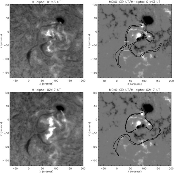
Figure 1. Left: Hα observations showing the filaments before (top) and after (bottom) their interaction. Ribbons of the simultaneously occurring flares are visible. Right: filament shapes overlaid on the MDI magnetogram taken at 01:39 UT (shapes drawn by eye after co-alignment). The white square outlines the area where the magnetic flux was measured (see Section 2 for details).
Download figure:
Standard image High-resolution imageTwo elongated filaments were present in the southeast of the AR, with their middle sections oriented in the north–south direction. At ≈ 1 UT, about 45 minutes before the onset of the main flare phase, these sections started to approach each other with a velocity of ≈10 km s−1. During the main phase (≈ 1:45–2:15 UT), the filaments collided, merged, and disconnected again. After this dynamic interaction, their middle sections were oriented east–west, i.e., the filaments had exchanged their footpoint connections.
Chandra et al. (2010) suggested that the flare and the filament interactions were not directly related, but were independent consequences of a global reconfiguration of the coronal magnetic field, driven by a nearby emerging and rotating bipole (the compact positive and negative polarities at the center of the magnetogram in Figure 1). They proposed that this continuous driving successively decreased the magnetic flux between the filaments, so that the filament-carrying fields approached and eventually reconnected with each other. To see whether such a flux decrease indeed took place, we measured the flux within the area marked by the white square in Figure 1, and found that the dominating positive flux decreased from ≈1.9 × 10¹⁹ Mx to ≈1.2 × 10¹⁹ Mx within about 5 hr before the flare and filament interaction. The photospheric magnetic field within the area is close to the noise level, so our measurements have to be taken with some care. Within this limitation, however, they support the scenario suggested by Chandra et al. (2010).
Independent of the detailed mechanism that was responsible for the approach of the filaments, their morphological evolution during their interaction suggests slingshot reconnection of the magnetic fields carrying the filament material, even though evidence of reconnection in terms of enhanced emission in the interaction region, and in the area magnetically connected to it, could not be observed (Chandra et al. 2010).
3. NUMERICAL SIMULATION
In order to model the observed filament dynamics, we follow the conjecture that filaments are located in magnetic dips. The exact geometry of the magnetic fields that support the filaments remains unknown for our event. Here, we choose a flux rope geometry and construct an initial field that contains two flux ropes oriented side by side. Since the exact mechanism which caused the approach of the filaments is unknown as well, we use ad hoc quasi-static boundary flows to bring the middle sections of the flux ropes into contact. We note that magnetic reconnection occurs in our simulation merely due to numerical diffusion; hence, we refrain from a quantitative investigation of the reconnection.
We employ the coronal flux rope model by Titov & Démoulin (1999, hereafter TD). It consists of a toroidal current ring of major radius R and minor radius a, with its center located at a depth d below a photospheric plane. The current is stabilized by placing two magnetic charges of strength ±q at the symmetry axis of the torus, at distances ±L from its center. A line current flowing along the symmetry axis is added to obtain a finite twist at the torus surface. Here, we omit the line current since it is not required for equilibrium (Roussev et al. 2003; Török & Kliem 2007). This yields a purely azimuthal magnetic field at the flux rope surface. The configuration above the photospheric plane is that of a twisted flux rope embedded in an arcade-like potential field.
3.1. Setup
We construct the initial magnetic field by superposing two TD configurations (Figure 2). The flux ropes are oriented along the y direction and placed at x = ±1.6. Guided by the footpoint locations of the filaments before and after their interaction (Figure 1), we choose the axial magnetic field By > 0 (<0) for the eastern, x < 0, (western, x > 0) flux rope. To account for the observed sign of photospheric flux surrounding the middle sections of the filaments, we choose the magnetic charges located between the TD tori to be positive. Hence, to enable equilibrium, the flux rope current has to flow from north to south (south to north) in the eastern (western) rope, yielding left-handed twist for both ropes. The normalized parameters are chosen identical for both TD tori: R = 2.75, a = 0.7, d = 1.75, |L| = 1, and |q| = 2.33, yielding a twist of ≈1.35 windings (averaged over the torus cross-section), which is below the threshold of the helical kink instability (Török et al. 2004).
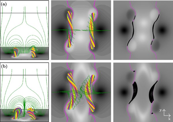
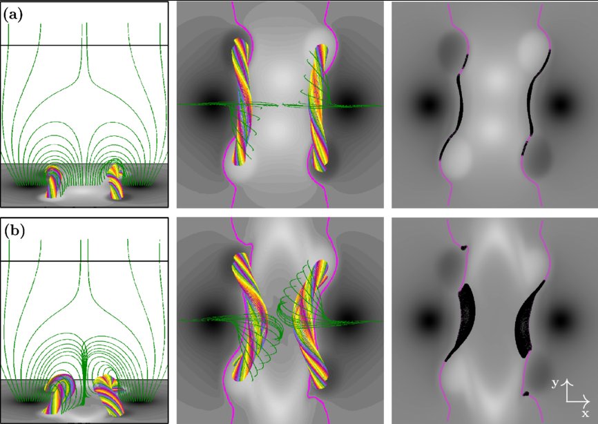
Figure 2. Numerical configuration after the initial relaxation (a) and after the diverging flow phase and subsequent relaxation (b). Bz(z = 0) is shown in grayscale with strong positive (negative) flux in white (black). Polarity inversion lines are drawn in pink. Left: oblique view along the flux ropes, showing their cores by rainbow-colored field lines and ambient field lines in green. Middle: top view. Right: top view, showing field line dips as black circles. The subdomain [ − 4, 4] × [ − 4, 4] × [0, 8] is shown in all panels.
Download figure:
Standard image High-resolution imageIn order to facilitate the diverging flows described in Section 3.2, we shift the positive charges away from y = 0, to y = −1 (1) for the eastern (western) flux rope. Furthermore, to obtain more compact photospheric potential field sources for the given TD parameters, we place all charges at a depth z = −d/2. To assure an approximate equilibrium after these modifications, we finally replace the above-mentioned values of q by 0.7 and −1.4 for the positive and negative charges, respectively. The final configuration (after numerical relaxation) is shown in Figure 2(a). The potential field is open at large heights and contains a null point at (0, 0, z = 4.7).
As in previous simulations of the TD model (e.g., Török & Kliem 2005), we integrate the zero β compressible ideal MHD equations, neglecting thermal pressure and gravity. The equations are discretized on a non-uniform Cartesian grid of size [ − 5, 5] × [ − 8, 8] × [0, 8], with almost uniform resolution Δ ≈ 0.04 where the flux ropes are located. The plane {z = 0} corresponds to the photosphere. The equations are normalized by the initial axis apex height of the TD tori, R − d, the maximum initial field strength,  , and the Alfvén velocity,
  , at the position of
  , (x, y, z) = (±2.64, 0, 0), and derived quantities. The Alfvén time is
  . The boundary conditions are as in Török & Kliem (2003), to which we refer for further numerical details. The initial density distribution is ρ0(x) = |B0(x)|3/2, such that va slowly decreases with the distance from the flux concentrations.
3.2. Photospheric Driving
We first relax the system for 114 τa. The resulting configuration (Figure 2(a)) shows no indication of dynamic behavior. We now have to bring the ropes into contact at their middle sections, for which we employ quasi-static flows at the bottom boundary.
Since the potential field between the flux ropes is unipolar and only weakly sheared (Figure 2(a)), driving the ropes toward each other would yield a pile-up of flux between them, hindering the ropes from coming into contact and reconnecting. Therefore, we first apply a diverging flow that moves the positive potential field polarities out of the area between the ropes. It also weakens the flux between them, as suggested by the observations (Section 2). To this end, we impose the following flow pattern in z = −Δz, within the area (|x| < 1.25, |y| < 6):

Here, um = 0.02 and ux,z(−Δz, t) = 0. The flow decreases smoothly to zero toward the edges of the area. Outside it, ux,y,z(−Δz, t) = 0. We use h(t) to linearly ramp the velocities up and down for 10 τa before and after the constant driving, respectively. The latter is applied for 110 τa. Afterward, the system is relaxed for 113 τa and time is reset to zero. The resulting configuration is shown in Figure 2(b).
In a second driving phase, we impose a similar flow pattern in z = −Δz, now within the area (|x| < 4, |y| < 1.5):
Here, um = 0.02 and uy,z(−Δz, t) = 0. Again, all velocities are zero outside the area. The flow is ramped up and down for 10 τa, respectively, and is constantly driven for 80 τa. This yields a converging flow of the negative potential field polarities, which slowly moves the flux rope middle sections toward each other. Afterward, the system is finally relaxed for 65 τa.
4. RESULTS AND DISCUSSION
In the course of the initial relaxation, the system evolves toward a numerical equilibrium that is similar to the analytical configuration. The flux ropes become slightly tilted toward the box center at their middle sections (Figures 2(a) and 4(a)) due to the slight asymmetry of the potential field surrounding each flux rope.
4.1. Diverging Flow Phase
During the diverging flow phase, the magnetic field between the flux ropes weakens and becomes increasingly sheared. As a consequence, the ropes expand slightly and lean toward each other (Figure 2(b)), and a localized vertical current layer forms between them, extending up to the region around the null point (Figure 4(b)). As the driving is stopped, the system relaxes toward a new numerical equilibrium in which the forces exerted by the ambient field on the flux rope currents and the repelling forces of these currents balance each other. The rope currents are very close to each other at their middle sections, divided by the current layer. Note that this layer is distinct from the flux rope currents. The current in the layer is directed primarily vertically, due to a change in sign across the layer of the horizontal component of the fields (Figure 2(b)). In contrast, the flux rope currents are directed primarily horizontally, parallel to the rope axes.
Figure 5 shows the evolution of the current densities in the lower section of the layer (where the flux ropes approach each other) during the driving phase and subsequent relaxation. The current densities grow exponentially, at an approximately constant rate, until the diverging flows are switched off, and do not change significantly afterward. They remain relatively weak, with the maximum current density in the layer reaching only about 15% of the maximum current density inside the flux ropes.
We checked different durations of the divergence flow phase. For too short durations, the field between the flux ropes does not get sufficiently weakened, and the converging flows applied later on lead to a strong pile-up of positive flux between the ropes, hindering their reconnection. Diverging flow phases longer than the one described here do not further weaken the field significantly, and the system evolves toward a configuration similar to the one shown in Figures 2(b) and 4(b). For the model settings considered here, converging flows hence appear essential for triggering reconnection.
The modeled filaments shown in Figure 2 seem to widen strongly during the diverging phase. This is due to the fact that dips typically form a thin vertical sheet within a flux rope (e.g., Dudík et al. 2008), and that the flux ropes here have oblong, rather than circular, cross sections. As the ropes lean to the side, so do the sheets of dips, which therefore appear to widen when seen from above. This effect might contribute to the frequently observed widening of filaments shortly before their eruption (see, e.g., Figure 3 in Gosain et al. 2009), if the flux rope carrying the filament material slowly rises in a direction inclined from the observer's line of sight.
4.2. Converging Flow Phase
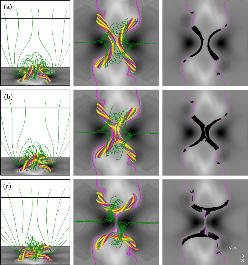
As the converging flows are applied, the evolving ambient field continuously pushes the flux ropes against each other, and the lower parts of the ropes are additionally pushed toward the box center by the imposed flows. However, although the flux ropes are already very close to each other before the onset of the converging flows (Figure 4(b)), they do not reconnect significantly with each other for about almost 60 Alfvén times (Figure 3(a)). This slow onset of reconnection can be explained by the fact that the field lines at the opposing rope surfaces are initially still almost purely azimuthal, hence almost parallel to each other, and therefore resist to reconnect. However, since the ropes are continuously driven together, they deform and the contact angle between the field lines slowly increases. This allows reconnection to set in, and the driving ensures that it continues even though the field line contact angle is initially small. Then, as the almost purely azimuthal outer field lines reconnect away, the contact angle between successively reconnecting field lines quickly increases and the reconnection accelerates, leading to the full splitting and reconfiguration of the ropes within ≈10 τa (Figure 3(b) and 3(c)). Since the flux ropes thereby fully exchange their footpoint connections, this reconnection is of slingshot type (Linton et al. 2001). Reconnection continues in the volume afterward, but in a less impulsive manner and without further affecting the flux rope connectivities.

Figure 3. Same as Figure 2, but during the converging flow phase, at times t = 58, 61, and 93 (a)–(c).
Download figure:
Standard image High-resolution image
Figure 4. Oblique view (top) and top view (bottom) on isosurfaces of current density with |j| = 0.1jmax, shown for the same domain as in Figures 2 and 3, and at the same times as in Figures 2(a), 2(b), and 3(c), respectively (a)–(c).
Download figure:
Standard image High-resolution imageThe evolution of the current densities in the lower part of the vertical current layer can be inferred from Figure 5. As the converging flows are applied, the current densities start to grow exponentially, now with a significantly larger growth rate than in the diverging flow phase. At t ≈ 60, around the time when the reconnection between the flux ropes accelerates, the maximum current density inside the layer has become about five times larger than the maximum value inside the flux ropes. Between t ≈ 50 and the onset of accelerated flux rope reconnection, the current densities undergo a phase of additional increase, which may be attributed to flux pile-up between the flux ropes as they fail to "adjust" to the continuous pushing by further deformation (a similar behavior of the current densities was observed in the simulations of kink-unstable flux ropes by Török et al. 2004, where the flux rope in the downward kinking case continuously pushed the current layer toward the rigid bottom boundary; see their Figures 3 and 4). After t ≈ 70, when the ropes have fully reconnected, the current densities in the layer slowly decrease as the system relaxes toward a new equilibrium.

Figure 5. Evolution of the current density in the vertical current layer as a function of time (in Alfvén times), shown at (x, y, z) = (0, 0, 0.6). The evolution is representative of the lower section of the current layer, where the flux ropes interact (see Figure 4). The duration of the driving and relaxation phases is indicated by vertical lines. The dashed line marks the onset of the converging flow phase, during which time has been reset to zero.
Download figure:
Standard image High-resolution image
We find slingshot reconnection between flux ropes with the same sign of twist. This contrasts with Linton et al. (2001), who found that ropes with a strongly azimuthal field at the surface and oppositely directed axial field bounce, without significant reconnection. This can be explained by the fact that the ropes in Linton et al. (2001) were not continuously driven together. Therefore, the reconnection did not have time to fully develop. In later simulations, however, with a weaker azimuthal field at the flux rope surfaces, and a correspondingly larger initial field line contact angle, Linton (2006) indeed found that slingshot reconnection can occur for flux ropes of the same sign of twist.
Figure 3 shows that the model filaments follow the morphological evolution of the flux ropes, hence qualitatively reproducing the observations (Figure 1). Mimicking the filaments by dip locations is actually not appropriate during the highly dynamic reconnection phase. However, since the system evolves almost quasi-statically before the reconnection, and relaxes toward a new equilibrium afterward (no indications of flux rope instabilities were found after the reconnection), calculating the dips before and after reconnection is sufficient to show that the model filaments exchanged their footpoint connections.
Here, we have used flux ropes with strong azimuthal fields at their surfaces to model the filament-carrying magnetic fields. We expect qualitatively similar results (i.e., merging and breaking) if suitably oriented sheared arcade fields (or weakly twisted flux ropes) were chosen instead, since the occurrence of slingshot reconnection is primarily due to the oppositely oriented axial fields in the (weakly twisted) cores of our reconnecting flux ropes. It can be expected, though, that the reconnection would set in much earlier for sheared fields, since the initial bouncing due to the almost parallel surface fields occurring in our simulation would be absent or much less pronounced. Accordingly, the evolution of the reconnection should be more strongly correlated with the photospheric driving, hence less impulsive and "slingshot-like." Sheared arcade fields may, however, not yield a sufficient number of field line dips after their reconnection to account for the observed filament pattern. Therefore, more sophisticated simulations (including a proper treatment of the coronal thermodynamics) may be required to test the ability of sheared arcade fields to reproduce the observed filament dynamics.
5. CONCLUSIONS
Our results support the suggestion by Kumar et al. (2010) and Chandra et al. (2010) that the dynamic interaction of the filaments on 2003 November 20 was due to magnetic reconnection between the filament-carrying magnetic fields, presumably flux ropes. In addition, these results provide a significant extension of the earlier work of Linton et al. (2001) and Linton (2006) on reconnection of convection zone flux ropes, by showing that slingshot reconnection can occur for coronal flux rope configurations as well. This study therefore provides proof of the concept that flux rope reconnection can be used to model and understand some coronal prominence interactions and the resulting dynamics.
We thank V. S. Titov and the anonymous referee for helpful comments. We also thank W. Uddin for his contribution in obtaining the Hα data shown in Figure 1. The research leading to these results has received funding from the European Commission's Seventh Framework Programme (FP7/2007–2013) under the grant agreement n 218816 (SOTERIA project, http://www.soteria-space.eu). Financial support by the European Commission through the SOLAIRE network (MTRM-CT-2006-035484) is also gratefully acknowledged. T.T. was partially supported by the NASA HTP and LWS programs. R.C. thanks the Centre Franco-Indien pour la Promotion de la Recherche Avancée (CEFIPRA) for his postdoctoral grant. The authors acknowledge financial support from CEFIPRA. C.H.M. thanks the Argentinean grants UBACyT X127 and PICT 2007–1790 (ANPCyT). C.H.M. is a member of the Carrera del Investigador Científico, CONICET. M.G.L acknowledges financial support from ONR and NASA grant NNO6AD58I, and thanks LESIA for hosting him during the 2010/11 academic year. The authors acknowledge financial support from ECOS-Sud (France) and MINCyT (Argentina) through their cooperative science program (N°A08U01).