


ABSTRACT
The magnetic field structure of the ejecta of a coronal mass ejection (CME) is not known well near the Sun. Here we demonstrate, with a numerical simulation, a relationship between the subsonic plasma flows in the CME-sheath and the ejecta magnetic field direction. We draw an analogy to the outer heliosphere, where Opher et al. used Voyager 2 measurements of the solar wind in the heliosheath to constrain the strength and direction of the local interstellar magnetic field. We simulate three ejections with the same initial free energy, but different ejecta magnetic field orientations in relation to the global coronal field. Each ejection is launched into the same background solar wind using the Space Weather Modeling Framework. The different ejecta magnetic field orientations cause the CME-pause (the location of pressure balance between solar wind and ejecta material) to evolve differently in the lower corona. As a result, the CME-sheath flow deflections around the CME-pauses are different. To characterize this non-radial deflection, we use  , where VN and VT are the normal and tangential plasma flow as measured in a spacecraft-centered coordinate system. Near the CME-pause, we found that θF is very sensitive to the ejecta magnetic field, varying from 45° to 98° between the cases when the CME-driven shock is located at 4.5 R☉. The deflection angle for each case is found to evolve due to rotation of the ejecta magnetic field. We find that this rotation should slow or stop by 10 R☉ (also suggested by observational studies). These results indicate that an observational study of CME-sheath flow deflection angles from several events (to account for the interaction with the solar wind), combined with numerical simulations (to estimate the ejecta magnetic field rotation between eruption and 10 R☉) can be used to constrain the ejecta magnetic field in the lower corona.
Export citation and abstract BibTeX RIS
1. INTRODUCTION
In this work, we draw an analogy between the outer heliosphere and interplanetary coronal mass ejections (ICMEs). There are commonalities between the two structures (see Figure 1, adapted from Opher 2010). The supersonic solar wind in the outer heliosphere passes through a shock, called the termination shock (TS), as it approaches the interstellar medium (ISM). The TS is located 85–95 AU from the Sun (Stone et al. 2005, 2008). The heliosheath is the region between the TS and the heliopause (HP; the contact discontinuity between the solar wind and the ISM). The subsonic solar wind propagates though the heliosheath and deflects around the HP. Similarly, an ICME can drive a shock ahead of it as it propagates away from the Sun. In the rest frame of the shock, a supersonic solar wind is shocked as it moves in the Sunward direction. This subsonic flow deflects around the magnetic ejecta at the contact discontinuity (we refer to this structure as the CME-pause). The CME-pause is the location of pressure balance between the shocked solar wind and the magnetic ejecta, and so it is analogous to the HP. Between the CME-pause and the CME-driven shock is the CME-sheath. Therefore, in the direction of solar wind flow away from the Sun, an ICME is like an inverted heliosphere (Figure 1).
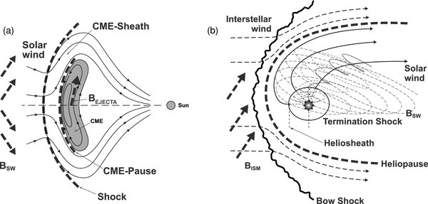
Figure 1. (a) An interplanetary coronal mass ejection (ICME) and (b) the outer heliosphere both present shock (CME-shock and termination shock) and sheath (CME- sheath and heliosheath) features. In this work, we draw on analogies between the two structures. The effect of the interstellar magnetic field (BISM in the outer heliosphere) corresponds to the effect of the magnetic field in the ICME (Bejecta). See the Introduction section (Section 1) for a detailed discussion. This figure has been adapted from Opher (2010).
Download figure:
Standard image High-resolution imageThe HP is distorted by the interstellar magnetic field pressure due to the compression of the magnetic field against the HP by the slowdown of the approaching interstellar flow. This slowing causes the magnetic pressure to dominate the thermal pressure close to the HP, forcing it to align with the interstellar magnetic field (Opher et al. 2007, 2009). The subsonic heliosheath flows downstream of the TS are immediately sensitive to the shape of the HP and therefore can probe the interstellar magnetic field direction (which is poorly constrained). The Voyager 2 spacecraft crossing of the TS (Stone et al. 2008) provided the first in situ data of the heliosheath flows. Opher et al. (2009) used a global simulation and Voyager 2 observations of heliosheath flows to constrain the interstellar field magnitude and direction.
The analogous quantity to the interstellar magnetic field in the ICME case is the ejecta magnetic field. The photospheric magnetic field from synoptic maps, specifically the neutral line of the source active region, is used to constrain the ejecta field direction near the Sun. The presence of a sigmoid can constrain the CME's orientation, as the material often aligns with the neutral line of the active region (Sterling et al. 2000; Gibson et al. 2002). However, the neutral line structure is often complex, especially for active regions which produce fast CMEs (Wang & Zhang 2008). Additionally, studies have found the ejecta's field orientation to lie both along and across the neutral line of the source active region (Zhao & Hoeksema 1998; Wood & Howard 2009). There is also an example of in situ flux rope signatures with no identifiable source active region (Robbrecht et al. 2009). Therefore, the features of an active region are not a conclusive diagnostic for the initial orientation of the ejected magnetic field. In this work, we propose CME-sheath flow deflections as an additional constraint.
Spacecraft such as Ulysses, the Advanced Composition Explorer (ACE), the Solar Heliospheric Observatory (SOHO), and the Solar Terrestrial Relations Observatory (STEREO) provide direct plasma data as some part of the ICME structure passes. A magnetic cloud (MC; subset of ICMEs) is categorized by low temperature, low plasma beta, and a strong rotation of a highly organized magnetic field (Burlaga et al. 1981). The observed rotation of the MC's magnetic field has been interpreted as a twisted flux rope (Goldstein 1983); however it has been argued that the rotation could instead be due to writhing of the field (Jacobs et al. 2009). Irrespective of whether the magnetic structure of an ICME is a twisted flux rope, flux rope models are successful in reproducing observational signatures (Forbes et al. 2006 and references herein). The orientation of a MC's flux rope axis can be estimated using minimum variance analysis (Bothmer & Schwenn 1998). The global magnetic structure of an ICME can be reconstructed with multiple spacecraft measurements using methods such as the Grad Shafranov reconstruction, from which the flux rope axis can be found (Yurchyshyn et al. 2007; Möstl et al. 2009).
The capability of CME-sheath deflection flows to indicate the geo-effectiveness of an ICME was investigated in Liu et al. (2008a). They found that the meridional deflection speed was well correlated to the ICME's speed (relative to the solar wind). As the meridional flow is coupled to the meridional magnetic field, the ICME speed observation was suggested to be used to predict the sheath magnetic field. Using a numerical simulation in which an eruption was set from the equatorial region, Manchester et al. (2005) characterized meridional flows in the CME-sheath. They identified the deflection of high-latitude sheath plasma toward the equator, which created a compression region behind the shock (stronger than the shock itself).
In a survey of non-radial solar wind flows from 1998 to 2002 ACE data, Owens & Cargill (2004) found that half of all large flow events were associated with ICMEs. Five events without complex deflection were studied in detail. The measured sheath flow deflection was in agreement with the inferred local ICME geometry (determined with variance analysis), demonstrating that the deflection measured by a spacecraft depends on the local axis of the flux rope, and the separation of spacecraft and the axis. Here, we use global magnetohydrodynamics (MHD) modeling to establish a relationship between the subsonic flows in the CME-sheath and the ejecta magnetic field orientation in the lower corona.
In global MHD modeling, coronal fields are commonly extrapolated from a Potential Field Source Surface model (Altschuler & Newkirk 1969), utilizing a line-of-sight synoptic magnetogram. When modeling a real space weather event, the magnetic field of the CME ejecta is a free parameter (Manchester et al. 2008; Kataoka et al. 2009; Lugaz et al. 2009; Cohen et al. 2010). Several analytic CME initiation solutions have been proposed (e.g., Dryer et al. 1979; Chen 1989; Forbes & Priest 1995; Lin et al. 1998; Gibson & Low 1998; Titov & Démoulin 1999; Antiochos et al. 1999; Krall et al. 2000). Some of these have been incorporated into numerical models of CME propagation (e.g., Linker et al. 2003; Roussev et al. 2004; Manchester et al. 2004; Lynch et al. 2004; Kunkel & Chen 2010). The main differences between the models are the geometry of the magnetic field and the physics of the trigger mechanism, such as reconnection, flux emergence, flare blast wave, and shear flows (Forbes et al. 2006). In this work, we do not attempt to validate any initiation mechanism. We simulate modified Titov–Demoulin (TD) flux ropes (Roussev et al. 2004) with the same initial free energy but different magnetic field orientations.
The evolution of an ICME is, in general, determined by two factors: properties of the ejecta (such as magnetic field geometry with respect to the coronal and active region fields), and the background solar wind in which it propagates (for example, Liu et al. (2006) showed that MCs are flattened by their interaction with the solar wind). The same background solar wind is used in each simulation, so in this work we do not account for different backgrounds. In the conclusion section, we discuss how an observational study of CME-sheath flow angles at 1 AU from several events (to remove the effects of the background), combined with numerical simulations can be used to constrain the ejecta orientation.
This manuscript is organized as follows: Section 2 provides an overview of the simulation and the CME model; Section 3 contains simulation results; and in Section 4 we provide discussion, conclusions, and future work.
2. METHODOLOGY
2.1. Background Solar Wind
To simulate the background solar wind, we use the Space Weather Modeling Framework (Tóth et al. 2005). The three-dimensional MHD code Block Adaptive Tree Solar-Wind Roe Upwind Scheme (BATS-R-US) which serves as its core is highly parallelized and includes adaptive mesh refinement. Cohen et al. (2008) validated solar wind parameters at 1 AU for many carrington rotation (CR), and CME simulations have used the same background solar wind and initiation mechanism as in this work (Liu et al. 2008b; Loesch et al. 2011; Cohen et al. 2010).
The simulation domain is a Sun-centered box of size 24 × 24 × 24 R☉ with six levels of refinement (each differing by a factor of two). There heliospheric current sheet is refined with cells of size 3/32 R☉. The initial solar magnetic field is calculated with the Potential Field Source Surface model (Altschuler & Newkirk 1969) and a Michelson Doppler Imager synoptic magnetogram for CR1922. This time frame corresponds to 1997 April–May (solar minimum), and so the global coronal field is a dipole. The solar wind is heated by a spatially varying polytropic index that also drives the wind's expansion (Cohen et al. 2007). The index is calculated with the Bernoulli integral, utilizing the Wang–Sheeley–Arge model (Arge & Pizzo 2000). It has a value close to 1 at the lower boundary and is equal to 1.5 above 12 R☉. After the flux rope is inserted into the background (which initiates the CME, see details below), the index profile is fixed to limit the exchange of heat between the CME and the background solar wind. The amount of background heating due to the spatially varying index was estimated in Evans et al. (2009).
2.2. CME Initiation
After the steady-state solution is achieved, a high resolution box containing cells of size 3/256 R☉ is placed in the path of the ICMEs' propagation. The rectangular box has dimensions of 1 R☉ in longitude, 1.8 R☉ in latitude, and extends to 6 R☉ in the ICME's path. The purpose of the box is to eliminate the influence of jumps in grid refinement on the ICMEs' evolution and capture the shock and ICME properties well near the nose. The total number of cells in the simulation domain is 12.4 × 10⁶.
A modified TD flux rope (Roussev et al. 2004) is inserted out of equilibrium in an active region near the equator (NOAA AR8038). This active region was the source region for the 1997 May 12 CME, which was Earth-directed (Thompson et al. 1998). As we have configured the TD flux rope, using only a line current running through the torus, the ejecta field is poloidal. The superposition of the polodial field with the coronal field produces an axial component to the flux rope field, in the −Z direction for Case A and the +Y direction for Cases B and C (see Figure 2(d)). The parameters of the flux rope model are: a torus radius of 0.14 R☉, cross section radius 0.03 R☉, mass 4.5 × 10¹² g, and torus line current 5 × 10¹¹ A (no subphotospheric magnetic charges or line current are included).

Figure 2. (a)–(c) Schematics to demonstrate the relative geometry of the ejecta field Bejecta, active region field Bar, and global coronal field Bcor in Cases A–C. The insets show the definition of β, the angle between Bejecta and Bcor. Bejecta is (a) perpendicular, (b) antiparallel, and (c) perpendicular to Bcor (which is in the −Z direction). Bar is along the +Y direction. (d) Initial configuration (from the simulation) for the ejecta for Case C inserted into AR8038. The solar surface is colored with the radial component of the magnetic field. The gray isosurface is current density  , which defines the surface of the flux rope, and the magnetic fields are labeled accordingly.
Download figure:
Standard image High-resolution imageWe set the initial magnetic field orientations by changing the location and direction of the torus line current. The flux rope chirality for Cases A and C is right-handed, whereas Case B is left-handed. The cases can be identified by the quantity β, which we have defined to be the angle between the poloidal field (Bejecta) and the coronal field (Bcor). The global coronal field is in the −Z-axis, active region is in the +Y-axis, and ICME propagation is in the +X-axis. The angle β for Case A is 90°, for Case B 180°, and for Case C 0°, as can been seen in the insets of Figures 2(a)–(c). We define another angle γ measured between Bejecta and the active region field Bar, which is 180° for Case A, −90° for Case B, and 90° for Case C.
All three CMEs contain the same initial free energy (2 × 1032 erg), launched into the same solar wind background with the same numerical resolution. Detailed analysis of the ICMEs' evolutions will be presented in a future study.
3. RESULTS
3.1. CME-pause
The CME-pause separates the shocked solar wind from the ejecta material and defines the region downstream of the sheath. Burlaga (1988) considered flux rope cases with different orientations with respect to the rotation axis of the Sun. It was shown that sharp changes in the angle  (where BZ is the rotation axis of the Sun and B is the magnetic field strength) approximately marked the edges of the flux rope. To define the front of the ejecta (the CME-pause) in our simulations, we consider the angle
where BN is the normal component of the magnetic field in the Radial–Tangential–Normal (R-T-N) coordinate system (a Cartesian system defined at the location of the spacecraft; R is the direction from the center of the Sun to the spacecraft location, T is in the direction R × Z (the solar rotation axis), and N completes a right-handed system). A strong change in this angle indicates the boundary between the sheath and ejecta magnetic fields. The boundary traced out by a jump in θB at the CME-pause coincided with an isosurface of temperature (log T = 6.8, T in K), which is shown for each case in Figure 3.

Figure 3. Isosurfaces of the CME-pause for (a) Case A, (b) Case B, and (c) Case C. The view is from a position along the +X-axis looking toward the approaching ICME, and the surface was defined as an isosurface of temperature (log T = 6.8, T in K). The contour gives magnetic field strength, and the black lines show the ejecta magnetic field inside the CME-pause. The white arrow indicates the direction of the CME-sheath deflection flows. The gray solid line indicates the trajectory of an artificial spacecraft, and the simulation times (a) 40 minutes, (b) 48 minutes, and (c) 56 minutes after the flux rope was inserted correspond to the CME-driven shocks reaching a height of 4.5 R☉ along this trajectory. Note the differences in the shape and size of the CME-pause.
Download figure:
Standard image High-resolution image
Figure 3 shows the CME-pause for each simulated ejection, viewed along the +X-axis looking toward the approaching ICME. The contour gives the magnetic field strength. The black lines show the ejecta magnetic field just inside the CME-pause (to show the different draping of the field around the CME-pause). The gray line indicates the path of an artificial satellite (draw radially from the center of the Sun), along which we measure the height of the CME-driven shock. At the intersection of the gray line and the CME-pause, the value for θB is: −69° (Case A), −10° (Case B), and −36° (Case C). The thick gray arrow indicates the direction of the sheath deflection flows in front of the pause (to be discussed in Section 3.2). The simulation times correspond to the shocks reaching a height of 4.5 R☉. The times in Figures 3 are (a) 40 minutes, (b) 48 minutes, and (c) 56 minutes after the flux rope was inserted.
We can see that the CME-pause shape is different for each case. The same trend was found in Opher et al. (2009), where the HP shape was sensitive to the pressure of the interstellar magnetic field ahead, aligning it with the direction of interstellar magnetic field. Just like in the outer heliosphere, the magnetic pressure of the ejecta near the CME-pause dominates the thermal pressure. The average ratio of thermal to magnetic pressure is 0.083 (measured inside the ejecta for the three cases when the CME-pause is located at 4.5 R☉). The location on the CME-pause where the magnetic field strength is intensified is different for the three ejecta field configurations. As a result, the CME-pauses are distorted differently for different ejecta field orientations. The ratio of the latitudinal extent of Case A : B : C is 1 : 1.1 : 0.6. The ratio of the longitudinal extent transverse to the spacecraft trajectory is 1 : 0.8 : 0.6. From the viewpoint in Figure 3, Case A is most circular and Case B has experienced more latitudinal expansion than longitudinal. Case C is most asymmetric and the smallest (from this perspective).
In the outer heliosphere, the HP axis was found to align with the direction of the local interstellar magnetic field (Opher et al. 2009). The ICME ejecta field is much less organized than the interstellar magnetic field, as seen in Figure 3, however the CME-pause shapes are in agreement with the ejecta flux rope axis.
3.2. Deflection of CME-sheath Flows
As a result of the bimodal solar wind, an indentation forms in the shock near the equator (Manchester et al. 2005). This dimple is caused by the magnetic field lines behind the shock bending toward the equator (over a short distance), resulting in a complex pattern of equatorial then poleward directed plasma flow behind the shock. Therefore, we sample flows at latitudes above the dimple, where the nonradial flow is only due to deflection away from the CME-pause. As discussed in the previous section, we define the CME-pause as a strong change in the angle  (Burlaga 1988). We also use θB to define the beginning of the sheath (downstream of the shock), as it also changes value suddenly at the boundary between the unshocked solar wind and sheath magnetic fields. The location of this change coincides with the jumps of the Rankine–Hugoniot relations.
In the previous section, we showed that the CME-pauses are different for the three cases. As such, we expect that the subsonic CME-sheath flow deflections away from the CME-pause will be different. For subsonic solar wind flows in the outer heliosphere, Opher et al. (2009) determined the parameter most sensitive to the direction of the interstellar magnetic field θF, where
Here, VN and VT are, respectively, the normal and tangential components of the plasma flow in the R-T-N coordinate system. We tested several plasma flow parameters and also found that θF was the quantity most sensitive to the ejecta magnetic field.
In Table 1, we provide the deflection angle θF for each case when the CME-driven shock position was 4.5 R☉ (measured along the artificial spacecraft trajectory shown as the gray line in Figure 3). In the first column of Table 1, we indicate the angle β for each case, where β is the angle between Bejecta and Bcor. The flow deflection θF is estimated at two positions in the CME-sheath (measured along the spacecraft trajectory): just downstream of the shock (second column) and just before the CME-pause (third column). We indicate the magnetic field angle θB at the CME-pause in the fourth column. Downstream of the shock, θF for each case does not differ significantly (ΔθF= 4°, 5°, and 9°). The effect of the different CME-pauses can be seen by looking at the flow angles in front of the pause, where (ΔθF= 45°, 53°, and 98°).
Table 1. Flow Angle for Different Ejecta Orientations (Rshock = 4.5 R☉)
| Case | β | θF at CME-shocka | θF at CME-pauseb | θB at CME-pauseb |
|---|---|---|---|---|
| A | 90° | −86° | −43° | −69° |
| B | 180° | −82° | 55° | −10° |
| C | 0° | −77° | 10° | −36° |
Notes. aValue taken just downstream of the shock when the shock position (Rshock) is 4.5 R☉. bValue taken inside the sheath, just in front of the CME-pause when the shock position (Rshock) is 4.5 R☉. See Figure 3.
Download table as: ASCIITypeset image
3.3. Rotation of Ejecta
The magnetic field of a flux rope will rotate during propagation in the lower corona as a result of the Lorentz force (Isenberg & Forbes 2007). Simulations utilizing the breakout model showed that the Lorentz force can lead to a flux rope magnetic field rotation of 40° within the first few solar radii of evolution (Lynch et al. 2009). The direction of rotation is given by the handedness of the flux rope: clockwise rotation for Case B (right-handed) and counterclockwise for Cases A and C (left-handed). An additional effect that causes rotation is reconnection with the overlying coronal fields, as shown in simulations by Cohen et al. (2010) and Shiota et al. (2010). Cohen et al. (2010) demonstrated that reconnection can cause the ejecta to rotate significantly (90°) in the first hours of propagation. The initial orientation of the ejecta field in relation to the coronal field dictates the amount of reconnection, and therefore evolution of the ejecta magnetic field. We showed in the previous section that the CME-pause shape is sensitive to the ejecta magnetic field, and therefore the different rotations of the ejecta field cause different evolutions of the flow deflection angle
In Table 2, we present the evolution of the deflection angle, θF, from 3 to 6 R☉. We extracted data from a velocity streamline which intersects the artificial spacecraft's trajectory (shown as a gray line in Figure 3) at the same location inside each ejecta. This method was chosen to ensure that we tracked the same location on the CME-pause at all times. For each case, we calculate the change in θF in time downstream of the shock as the CME propagates in the lower corona.
Table 2. Evolution of Flow Angle Downstream of the Shock
| Case | ΔθFa | ||
|---|---|---|---|
| Rshock = 3–4 R☉ | Rshock = 4–5 R☉ | Rshock = 5–6 R☉ | |
| A | 3° | 5° | 2° |
| B | 4° | 8° | 7° |
| C | 2° | 1° | 1° |
Note. aThe difference in the deflection angle (see Section 3.2) between the two heights.
Download table as: ASCIITypeset image
We find the strongest rotation occurs for Case B: between 5 and 6 R☉, the deflection angle changes by 7°. The initial ejecta field for this case was configured to be antiparallel to the global coronal field, resulting in the most the reconnection, which explains its continued rotation at 6 R☉. The deflection angle changes by the least amount for Case C: only 1° from 4 to 5 and 5 to 6 R☉. The initial ejecta field for this case was configured to be parallel to the global coronal field, a less favorable arrangement for reconnection. Additionally, the strength of the magnetic field at the CME-pause for Case C is stronger, and the CME-ejecta expanded less, than Cases A and B. This indicates that it experienced the least reconnection (see Figure 3). The rotation for Case A, whose initial ejecta field was oriented perpendicular to the coronal field, is intermediate between Cases B and C. The change in the deflection angle is 5° between 4 and 5 R☉, showing that it is still undergoing rotation at this height. However, the rotation for Case A is less from 5 to 6 R☉ (ΔθF = 2°), implying that the ejecta's rotation is slowing.
4. DISCUSSION AND CONCLUSIONS
The goal of this work was to establish the subsonic CME-sheath deflection flows as a diagnostic for the ejecta magnetic field orientation in the lower corona. We chose three initial CME magnetic field orientations and performed highly refined, global MHD simulations in a background solar wind. The initial magnetic field of the ejecta for two cases is along the polarity inversion line of the source active region, while the third is across the active region. We selected these orientations to align with conjectures of ejecta magnetic field geometry based on observations (Zhao & Hoeksema 1998). All cases had the same initial free energy and were launched into the same solar wind. Because of the different orientations, the evolutions of the ICMEs differed. The details will be presented in a future study (Evans et al. 2010).
The analysis of CME-sheath flows was motivated by an analogy to the outer heliosphere. In both cases, since the sheath flows are subsonic, they deflect around the obstacle ahead (the pause). The pauses are affected by the dominant magnetic field. For the outer heliosphere, the HP is sensitive to the direction of the interstellar magnetic field because the magnetic pressure from the ISM pushes in on and shapes the HP. By using Voyager 2 heliosheath deflection flow data, Opher et al. (2009) were able to constrain the interstellar magnetic field. In this work, we found that the CME-pause size and shape are extremely sensitive to the ejecta magnetic field orientation. The magnetic pressure from the ejecta pushes out on and shapes the CME-pause. The deflection flows in the CME-sheath are sensitive to the pause, and so deflection angles measured by the same spacecraft for our three simulation cases are distinguishable from each other (ΔθF = 45°–98° at the CME-pause). This demonstrates that the flows are sensitive to the ejecta magnetic field.
We find that the flow deflection angle evolved with height until 6 R☉. The source of this evolution is the rotation of the ejecta due to the Lorentz force (Lynch et al. 2009) and magnetic reconnection (Cohen et al. 2010). The initial orientation (and magnitude) of the ejecta field in relation to the coronal field determines the amount of rotation in the lower corona. We found the evolution of θF diminishes as the CME propagates: for two of the cases, the change was less than 2°/R☉ when the CME-driven shock was located at 6 R☉. These results are in agreement with an observational study by Yurchyshyn et al. (2009). They found, using the Large Angle Coronagraph-Spectrograph (LASCO) white light images, that most flux ropes rotate by only about 10° above 6 R☉. Further, the 2008 April 26 CME event (reconstructed with a geometric model) did not have flux rope orientation evolution during propagation (Wood & Howard 2009). If the ejecta field does not undergo significant rotation after 10 R☉, then θF at the same location on the CME-pause would be frozen-in during propagation through the heliosphere, relating a lower corona quantity to a measurable quantity in the heliosphere.
The evolution of the CME-sheath flows is related to the evolution of the ICME, which is determined by two factors: the ejecta's properties and the background solar wind in which it propagates. In this work, we launched all ejections into the same background with the same initial free energy, differing only in the initial orientation of the ejecta field. We demonstrated that the flow deflection angle θF measured in the sheath is sensitive to direction of the ICME's magnetic field. This indicates that an observational study of CME-sheath flow deflection angles at 1 AU from several events (to account for the interaction with the solar wind), combined with an estimate of the ejecta magnetic field rotation between the eruption and evolution to 10 R☉—from simulations such as those of Lynch et al. (2009), Cohen et al. (2010), Shiota et al. (2010), and observations such as Yurchyshyn et al. (2007)—can be used to constrain the ejecta magnetic field in the lower corona.
It is important to emphasize that the deflection angle that a spacecraft measures depends on the separation of the spacecraft and the flux rope axis, or the stagnation point on the CME-pause. This point was demonstrated in the work of Owens & Cargill (2004). This effect was also seen by Opher et al. (2009) in the outer heliosphere, when using the heliosheath flow deflection measured by Voyager 2 (in that case the interstellar field determines the HP axis direction). Therefore, the deflection flows are sampling two effects: the distance to the stagnation point and the direction of the ejecta magnetic field.
The authors thank NASA Ames for the use of the Pleiades supercomputer, and an anonymous referee for comments that improved the manuscript. This work was supported by NSF Career Grant ATM 0747654.