THE DEUTERIUM-BURNING MASS LIMIT FOR BROWN DWARFS AND GIANT PLANETS

David S. Spiegel; Adam Burrows; John A. Milsom

doi:10.1088/0004-637X/727/1/57

1. INTRODUCTION

The year 1995 heralded both the first unambiguous detection of a brown dwarf (Oppenheimer et al. 1995) and the first unambiguous detections of planets beyond our solar system (Mayor & Queloz 1995; Marcy & Butler 1996). Many of the first substellar objects detected were either clearly brown dwarfs (very massive, not in a close orbit around a main-sequence star) or clearly planets (lower mass, orbiting close to their stars). However, as the number of discoveries of substellar objects grew to the dozens and then hundreds, there increasingly appeared to be overlap in the apparent mass distributions of brown dwarfs and planets. This highlighted the need to clarify the taxonomy. Moreover, the various definitions have been strained by the recent discoveries of objects such as CoRoT-3b, a ∼22 Jupiter-mass (M_J) object in a close (0.057 AU) orbit around its star (Deleuil et al. 2008) and the directly imaged objects of masses ∼5–15 M_J at tens of AU from HR 8799 and Fomalhaut (Marois et al. 2008; Kalas et al. 2008).

A commonly used way to classify objects that are ∼10–15 times the mass of Jupiter is by whether they fuse deuterium (D) in their deep interiors. This criterion was adopted in 2002 by the Working Group on Extrasolar Planets of the International Astronomical Union (Boss et al. 2007).

1.
Objects with true masses below the limiting mass for thermonuclear fusion of deuterium (currently calculated to be 13 Jupiter masses for objects of solar metallicity) that orbit stars or stellar remnants are "planets" (no matter how they formed). The minimum mass/size required for an extrasolar object to be considered a planet should be the same as that used in our solar system.
2.
Substellar objects with true masses above the limiting mass for thermonuclear fusion of deuterium are "brown dwarfs," no matter how they formed nor where they are located.
3.
Free-floating objects in young star clusters with masses below the limiting mass for thermonuclear fusion of deuterium are not "planets," but are "sub-brown dwarfs" (or whatever name is most appropriate).

Although we (and others) do not necessarily endorse the "deuterium-burning edge" as the most useful delineation between planets and brown dwarfs³ (see Burrows et al. 2001; Chabrier et al. 2005; and Bakos et al. 2010), it is a commonly used criterion and warrants further exploration.

Models of brown dwarfs and giant planets have been calculated since before the first such objects were discovered (Kumar 1963; Zapolsky & Salpeter 1969; Grossman & Graboske 1973; Burrows et al. 1993, 1995; Saumon et al. 1994). Such computations depended heavily on the equation of state (EOS) and were therefore aided by the publication of a new EOS for H₂–He mixtures (Saumon et al. 1995, the so-called SCvH EOS). In addition, models of the emergent radiation from, and of the temporal evolution of, brown dwarfs were improved by the application of non-gray radiative transfer theory (Burrows et al. 1997, 1998; Burrows & Sharp 1999; Burrows 1999; Burrows et al. 2001, 2003; Baraffe et al. 2002, 2003; Allard et al. 2003; Chabrier et al. 2000a, 2000b; Chabrier & Baraffe 2000; Sharp & Burrows 2007; Barman 2008) and sophisticated chemical models (Fegley & Lodders 1994; Lodders & Fegley 2002; Burrows & Sharp 1999; Sharp & Burrows 2007; Allard & Hauschildt 1995).

The theoretical study of brown dwarfs and massive planets is now a maturing field that is of particular current interest, given the increasing pace of discovery of objects in this mass range. Previous model calculations have suggested that deuterium burning turns on near a mass of 13 M_J (Burrows et al. 1997, 2001) or at 0.012 M_☉ (∼12.5 M_J; Chabrier et al. 2005).⁴ An early such calculation was performed by Grossman & Graboske (1973), who claimed the existence of a deuterium main sequence near 0.012 M_☉, although Dantona & Mazzitelli (1985) found, using a lower deuterium abundance, that there is no deuterium main sequence. The models of Grossman & Graboske (1973) used a deuterium fraction that was about 10 times the Galactic value, and the atmosphere treatment was less sophisticated than the current state of the art. Although previous calculations, and community prejudices, have converged on a mass limit of ∼13 M_J, and this mass range does provide a reasonable estimate for the mass at which significant deuterium burning occurs, it is worthwhile to clarify the precise range of deuterium-burning mass predictions under a variety of model assumptions. Saumon & Marley (2008) have contributed to this endeavor. Specifically, defining the minimum deuterium-burning mass as objects that burn 90% of their initial deuterium in 10 Gyr, they find 13.1 and 12.4 M_J for the cloudless and cloudy cases, respectively. This shows that how one computes the radiative boundary condition (with or without clouds, and what type of clouds) matters significantly.

In this paper, we systematically explore how deuterium burning depends on a several physical properties of objects. Our goal in this paper is to point out that the division between objects that burn deuterium and those that do not is not strictly 13 M_J. One important aspect of this is that deuterium burning does not "turn on" suddenly at a particular mass. Even with just a single set of model parameters, the mass at which 10% of deuterium burns is different from the mass at which 50% or 90% burns. This ambiguity is only enhanced when one examines the range of possible or likely values of the variables under consideration here (such as helium abundance, initial deuterium abundance, and metallicity). We consider various (cloud-free) models and nuclear burning criteria; in Section 2, we describe the models under consideration. We vary the helium fraction as a proxy for the effect of varied concentrations of elements heavier than hydrogen (Section 2.2); we vary the initial fraction of deuterium (Section 2.3); and we vary the metallicity in the context of its influence on atmospheric opacity and cooling (Section 2.4). In Section 3, we describe the influence that each aforementioned knob has on deuterium burning, and in Section 4, we calculate derivatives of the D-burning mass edge with respect to each quantity (Y, y_D,i, Z). In Section 5, we conclude by discussing the implications of our results for the distinction between brown dwarfs and giant planets.

2. MODELS

We consider a range of brown dwarf/planet models. If the objects are massive enough, their deep interiors have conditions under which non-negligible burning of deuterium occurs through the reaction p + d → γ + ³He (by far the most important reaction involving deuterium at the temperatures and densities in the cores of these objects). The rate of deuterium burning depends on the concentration of deuterium, the mass density, and the temperature. Stahler (1988) presents a power-law approximation to this rate in the range T ∼ 10⁶ K: epsilon _D ∝ ρy_DT^11.8, where epsilon _D is the specific deuterium-burning rate, ρ and T are central values of density and temperature, and y_D is the deuterium mixing ratio. Although this expression does not, of course, describe the actual deuterium-burning rate used in our code, it may serve as a rough guide. We vary the helium mass fraction (Y, which influences the central density), we vary the initial deuterium mixing fraction (y_D,i), and we vary the metallicity of the atmosphere (Z, which strongly affects the opacity). Our models are described in Sections 2.1–2.4 below and summarized in Table 1. Note that each row of this table actually corresponds to a family of models with a dense spacing of masses, ranging from 10 to 20 times Jupiter's mass.

Table 1. Models

Model	Z	y_D,i	Y	M (10%)	M (50%)	M (90%)
	(Z_☉^a)			(M_J)	(M_J)	(M_J)
He22	1	2 × 10⁻⁵	0.22	13.20	14.08	14.92
He25 (D2)^b	1	2 × 10⁻⁵	0.25	12.70	13.55	14.35
He28	1	2 × 10⁻⁵	0.28	12.06	12.83	13.62
He30	1	2 × 10⁻⁵	0.30	11.62	12.42	13.20
He32	1	2 × 10⁻⁵	0.32	11.32	12.05	12.78
D1	1	1 × 10⁻⁵	0.25	12.71	13.74	14.55
D2 (He25)	1	2 × 10⁻⁵	0.25	12.70	13.55	14.35
D4	1	4 × 10⁻⁵	0.25	12.45	13.09	13.93
Z0	0	2 × 10⁻⁵	0.22	14.37	15.40	16.30
Z0.01	0.01	2 × 10⁻⁵	0.22	13.59	14.56	15.39
Z0.1	0.1	2 × 10⁻⁵	0.22	12.92	13.82	14.65
Z0.3	0.3	2 × 10⁻⁵	0.22	12.48	13.33	14.14
Z1.0^c	1	2 × 10⁻⁵	0.22	12.00	12.79	13.56
T0.3	10^−1/2	1 × 10⁻⁵	0.25	12.92	13.77	14.67
T1	1	2 × 10⁻⁵	0.25	12.54	13.48	14.33
T3	10^1/2	4 × 10⁻⁵	0.25	12.20	13.13	13.86

Notes. Models He22–He32 and D1–D4 are calculated with a Burrows et al. (1997) radiative boundary condition Models Z0.01–Z1.0 are calculated with opacities from Allard & Hauschildt (1995), incorporated in atmospheric boundary conditions as described in Burrows et al. (2001) (D. Saumon 2001, private communication). Models T0.3–T3 have radiative boundary conditions calculated with COOLTLUSTY. Model Z0's radiative boundary condition comes from Saumon et al. (1994). ^aOur adopted value of Z_☉ = 0.0189 is taken from Anders & Grevesse (1989). This is in contrast to the 0.0142 value from the more recent work of Asplund et al. (2009). In absolute units, the quantities in the table correspond to the following values: 0 × Z_☉ = 0; 0.01 × Z_☉ = 1.89 × 10⁻⁴; 0.3 × Z_☉ = 0.00598. ^bThis model shows up in two rows, named both He25 and D2, and is one of two "fiducial" models. ^cThis is the other "fiducial" model.

Download table as: ASCII Typeset image

2.1. Modeling Technique

The basic modeling strategy is the one described in Burrows et al. (1997). Specifically, we self-consistently calculate the evolution of these objects by matching radiative-convective atmosphere models onto fully convective interiors. Objects are assumed to be born high on the Hayashi track, with a given high interior entropy and a flat entropy profile. This is a reasonable assumption because in Nature these objects become fully convective and lose their initial conditions (i.e., the entropy decreases rapidly from its initial high value) within 10³– 10⁵ years after formation. This is far shorter than the duration or age of deuterium burning, which can last 10⁷–10⁹ years. Interior structure is calculated with the SCvH EOS (Saumon et al. 1995). In the atmosphere, convective heat flux is treated with mixing length theory (Mihalas 1978), taking the mixing length to be the pressure scale height. Burrows et al. (1989) investigated how other choices of mixing length affect the thermal evolution of brown dwarfs and low-mass stars and found that, for brown dwarfs, unlike for stars on the main sequence, this dependence is very weak.

At temperatures found in the interiors of these objects, the rate of proton–deuteron fusion is reported in the literature as the standard extrapolation from the rates at higher temperatures. We use the rate reported by Caughlan & Fowler (1988), which is the same as that found in Harris et al. (1983). In 1999, the Nuclear Astrophysics Compilation of REaction rates (NACRE) released a new compilation of thermonuclear rates (Angulo et al. 1999), which was updated several years later (Descouvemont et al. 2004). Still, the recent release of the Reaclib Database (Cyburt et al. 2010) by the Joint Institute for Nuclear Astrophysics (JINA) uses the Caughlan & Fowler (1988) rate. A good discussion of nuclear fusion rates can be found in Adelberger et al. (2010). The Caughlan & Fowler rate and that of Descouvemont et al. (2004) differ by ∼20% at T ∼ 10⁸ K, and start to converge at lower temperatures. The interiors of these substellar-mass objects reach temperatures of ∼0.5–1 × 10⁶ K, where the Gamow peak energies are ∼0.7– 1 keV. At these temperatures and energies, the discrepancy between the older and the newer estimates of the rate is less than 10%, although extrapolations in this regime are generically problematic. To our knowledge, there is no newer information on how properly to make this extrapolation to temperatures and Gamow peak energies of relevance to the question at hand.⁵ Screening corrections for both ions and electrons are employed (Saumon et al. 1996; Dewitt et al. 1996; Sahrling & Chabrier 1998).

The thermal evolution depends on the cooling rate as a function of object size and entropy. In order to calculate this, as in Burrows et al. (1997), we pre-calculate a large grid of one dimensional, non-gray, radiative-convective atmosphere models with different effective temperatures (T_eff) and surface gravities (g). The effective temperature specifies the net radiative-convective flux at every vertical level (σT⁴_eff, where σ is the Stefan–Boltzmann constant). Each model in the grid is fully convective at its base. The grid of atmosphere calculations, therefore, can be thought of as defining a function S[T_eff, g], where S is the entropy. What is important for the thermal evolution is the net cooling rate (essentially T_eff). Therefore, we invert this function to obtain T_eff[S, g]. This function depends on the atmospheric opacities and is what is meant by the "surface boundary condition." At every step of the thermal evolution, the cooling rate is calculated by interpolating in the grid. In this way, the fully convective interior matches smoothly onto the appropriate atmospheric boundary condition.

2.2. Helium Fraction

For an ideal gas, density depends on molecular weight, while for degenerate matter, density is inversely related to the ratio of electrons to baryons. The abundance of heavier-than-hydrogen elements affects the density for both reasons. We vary the helium content of our models from Y = 0.22 to Y = 0.32, with more helium-rich models representing objects that are richer in both helium and metals. The corresponding model names (in Table 1 and in the figures) are He22–He32. Model He25 has helium mass fraction 0.25, and is also referred to as model D2 (described in Section 2.3). These models have a radiative boundary condition (i.e., atmospheric opacities) calculated using the method of Burrows et al. (1997), with solar-metallicity opacities and initial deuterium number fraction of y_D,i = 2 × 10⁻⁵.

We note that not all helium abundances are equally likely. Historically, quite low values of Y have been inferred for Jupiter and Saturn. Using two different instruments on Voyager, Gautier et al. (1981) estimated that the helium mass fraction of Jupiter was 0.19 ± 0.05 or 0.21 ± 0.06, respectively. More recently, von Zahn et al. (1998) used Galileo data to find the helium mass fraction of Jupiter to be 0.234 ± 0.005. In a reanalysis of Voyager data, Conrath & Gautier (2000) found the abundance in Saturn to be in the range 0.18–0.25. One must keep in mind that, because of differentiation, atmospheric values for these objects might be lower than bulk abundances. Furthermore, the Wilkinson Microwave Anisotropy Probe (WMAP) indicates that a fairly stringent lower bound on the cosmic primordial helium mass fraction is 0.248 (Spergel et al. 2007). Higher values than this can easily be explained in some objects from Galactic enrichment, but lower values might be difficult to explain. Nevertheless, we examine the effect of very low values of Y, down to 0.22, so as to explore the dependence of the deuterium-burning edge on Y values that have been invoked in the last several decades, but the reader should note that such an extreme value might not obtain in actual substellar objects.

2.3. Initial Deuterium Fraction

Big-bang nucleosynthesis calculations, in conjunction with other observations (cosmic microwave background (CMB), high-z quasars, etc.) suggest that the primordial D:H ratio is (2.8 ± 0.2) × 10⁻⁵ (Pettini et al. 2008). Our galaxy, however, is somewhat depleted in deuterium, relative to this value. Recent observations indicate that the mean mixing ratio of deuterium in the interstellar medium is roughly (2.0 ± 0.1) × 10⁻⁵, though the scatter (among different lines of sight) is a factor of several (Prodanović et al. 2010). In our models, we take initial deuterium fractions of 10⁻⁵, 2 × 10⁻⁵, and 4 × 10⁻⁵ (mixing ratios).⁶ The corresponding model names are D1, D2, and D4. These models also have a radiative boundary condition (i.e., atmospheric opacities) calculated using the method of Burrows et al. (1997), with solar-metallicity opacities and a helium mass fraction of 0.25.

2.4. Metallicity

For a non-irradiated object, the metallicity, i.e., the abundance of elements heavier than helium, is the main determinant of the atmospheric chemistry and, hence, the opacity.⁷ Among objects with thick H₂–He-dominated atmospheres, this abundance can range from very low, to more than 30 times the solar abundance, as is expected for objects such as Uranus, Neptune, and similar-mass exoplanets (Guillot & Gautier 2007; Spiegel et al. 2010; Lewis et al. 2010; Nettelmann et al. 2010; Madhusudhan & Seager 2010). Still, objects as massive 10 M_J might generally be expected to have metallicities not much more than 0.5–1 dex more than solar.

In our models, we take metallicity values ranging from zero up to a half dex more than solar, and we calculate the opacity corresponding to equilibrium chemistry (Burrows & Sharp 1999; Sharp & Burrows 2007). Here, we take solar metallicity to be defined by Anders & Grevesse (1989). The typical derived atmospheric molecular opacities and, hence, the net cooling rate resulting from these older abundances generally do not differ much from those calculated using the more recent Asplund et al. (2009) values, and the latter remain controversial. Furthermore, we point out that using the older elemental abundances is no obstacle to our basic goal, which is to explore the broad consequences of different metallicities on thermal evolution. Since other stars have different elemental ratios than the Sun, the degree of uncertainty in how our mix of elements matches that of typical stars depends at least as much on variability in typical stellar values as on the estimate of solar abundances. In the zero-metallicity models, atmospheric opacity results entirely from collisionally induced absorption due to the collisionally induced dipoles of H₂ and He (Borysow et al. 1989). Though the bottom end of this range (0 and 0.01 times solar) includes lower metallicities than might not be expected in most brown dwarfs, it is interesting to consider the full range of possibilities.

The models in which we vary metallicity fall into two sequences, Z0.01, Z0.1, Z0.3, Z1.0, and T0.3, T1, T3. Models in the former sequence are calculated using the opacities of Allard & Hauschildt (1995) to derive the atmospheric boundary conditions (D. Saumon 2001, private communication) that drive the evolution. These models have a helium mass fraction of 0.25 and initial deuterium fraction of 2 × 10⁻⁵. The metallicity of these models (as a fraction of solar) is the number following the Z in the model name. Those in the latter sequence have a boundary condition calculated using COOLTLUSTLY (Hubeny 1988; Hubeny & Lanz 1995; Hubeny et al. 2003; Burrows et al. 2006; Sharp & Burrows 2007), with the same helium and initial deuterium fractions K. Heng & A. Burrows (2011, in preparation). Among these, the metallicities of T0.3 and T3 are not exactly 0.3 and 3, but instead 10^−1/2 and 10^1/2 times solar metallicity. Finally, model Z0 has zero metallicity and is grouped by label with the former sequence, but actually has a radiative boundary condition taken from Saumon et al. (1994).

3. RESULTS

By considering a range of model parameters (Y, y_D,i, Z) and atmospheric radiative boundary conditions, and by examining evolutionary trajectories for a range of masses, at ages from 1 Myr to 10 Gyr, we have produced a broad range of model calculations. Here, we show how properties such as radius, effective temperature, and the deuterium-burning rate and power vary with time as a function of mass (Section 3.1). Furthermore, we examine how these evolutionary tracks vary with the other parameters at fixed mass (Section 3.2), and we calculate the variation of the deuterium-burning mass limit with the model parameters listed above (Section 3.3).

3.1. Evolution with Mass

The basic character of brown dwarf cooling trajectories is well known from a number of calculations in the last several decades, but it is worthwhile to examine the specific behavior of our models. We begin with an illustrative set of evolutionary trajectories for a representative family of models (He25 or D2). Figure 1 shows the evolution of four quantities that our models track.

The top panels show quantities related to model cooling. The top left panel shows the evolution of radius with time, and the top right panel shows the evolution of effective temperature with time. It is instructive to examine these two panels together. Higher mass objects begin larger but have higher effective temperatures and therefore cool more rapidly. As a result of their faster cooling, the radii of more massive objects shrink more rapidly, eventually (after roughly a gigayear) overtaking lower mass objects in radius. By the end of the calculation (after 10 Gyr), all objects are very nearly Jupiter's radius, but more massive objects are slightly smaller.

The lower panels of Figure 1 are related to the fusion of deuterium. During the initial Hayashi-track stages of evolution, the luminosity is dominated by Kelvin–Helmholtz contraction. After a few million years, the central part of the object reaches temperatures and densities at which the deuterium fusion rate is non-negligible. The bottom left panel shows the ratio of the power from nuclear (deuterium) burning to the total luminosity. For the most massive objects, this ratio reaches fairly large values (well over 80%). However, the main sequence is where this ratio is essentially 100% (i.e., where Kelvin–Helmholtz contraction has ceased), and so it is clear that none of these models goes through a deuterium main-sequence stage. The bottom right panel shows the evolution of the fraction of the initial deuterium (in this case, y_D,i = 2 × 10⁻⁵) that has burned. Higher mass objects burn a larger fraction of their initial deuterium, and do so faster than lower mass objects. Regardless of mass, very little deuterium burns after a few hundred million years. Note, in comparing the top row to the bottom row, that the 15 M_J and 20 M_J models, which fuse the greatest amount of deuterium (among the models displayed), cool and shrink very quickly after the deuterium-burning phase.

3.2. Model-dependence of D-burning Evolution

In Figure 2, we examine the deuterium-burning evolutionary profiles of 13 M_J objects from a variety of models. Each row shows analogous plots to the bottom row of Figure 1, only instead of different curves representing different mass objects, they represent different model properties. The left column shows the evolution of the ratio of nuclear power to total luminosity, and the right column shows the fraction of the initial deuterium that burns. The three rows show, from top to bottom, models He22–He32 (varying helium fraction), models D1–D4 (varying initial deuterium fraction), and models Z0–Z1.0 (varying metallicity through its influence on atmospheric opacity). Each row also shows models He25 (which is also D2) and Z1.0, for comparison to "fiducial" models.

First, it is important to note the difference at fixed model parameters of the radiative boundary condition. The Z-sequence models have higher opacity, which leads to slower cooling, than the other models (which have the Burrows et al. 1997 boundary condition). As a result, models Z1.0 and He25/D2, which are otherwise identical, have markedly different evolutionary trajectories. The former reaches a peak nuclear-to-total power ratio of ≈80%, while the latter reaches only ≈50%. Furthermore, the former eventually burns 66% of its initial deuterium, while the latter burns only 17% of its. In fact, of the Z-sequence models, model Z0.3 (with 0.316 × solar elemental abundance) more nearly approximates the He25/D2 evolution than does Z1.0. With its slower cooling, model Z1.0 has a moderate nuclear burning to total luminosity ratio until later times; the ratio shown in the left column stays above 5% until ∼5 Gyr.

More generally, within each row of Figure 2, the expected trends hold. The top row shows that more helium-rich models burn a greater fraction of their initial deuterium, which is unsurprising because these are the models with fewer electrons to support the mass via degeneracy pressure; thus, these models have denser, hotter cores. The middle row shows that models with higher initial deuterium content burn a greater fraction of their initial deuterium. This is a somewhat subtle point. The deuterium-burning rate is roughly linear in y_D, suggesting that, other things being equal, the fractional depletion of deuterium with time should be constant irrespective of initial deuterium abundance. However, other things are not equal. In particular, the central temperature of more deuterium-rich models is maintained at a higher value for a longer period of time. As a result, the integrated fractional amount of deuterium burned is greater for these models. The bottom row shows that more metal-rich models burn a greater fraction of their initial deuterium, which stands to reason because their higher opacities produce a blanket effect, allowing them to maintain higher core temperatures for a longer time.

3.3. Model-dependence of D-burning Limit

We now quantify the deuterium-burning mass limit and its dependence on the various model parameters we have varied. Figure 3 displays the same basic information in two different ways. In the left column, the fraction of the initial deuterium that combusts within 10 Gyr is plotted versus object mass. Horizontal dashed lines are plotted at 10%, 50%, and 90%, illustrating various (arbitrary) deuterium-burning cutoffs. The right column plots the deuterium-burning mass edge for each of these three criteria (i.e., the mass at the intersection of each curve in the left column with the corresponding dashed line) as a function of the three tunable model parameters: Y, y_D,i, and Z. From top to bottom, the rows show the same respective model sets as in Figure 2. As in Figure 2, models He25/D2 and Z1.0 are shown in all three panels of the left column. The last three columns of Table 1 contain the same information as the right column of Figure 3, and also include data for the COOLTLUSTY sequence of models (T0.3–T3). Note that the solar-metallicity COOLTLUSTY model (T1) and the fiducial Burrows et al. (1997) model (He25/D2) are quite similar to one another.

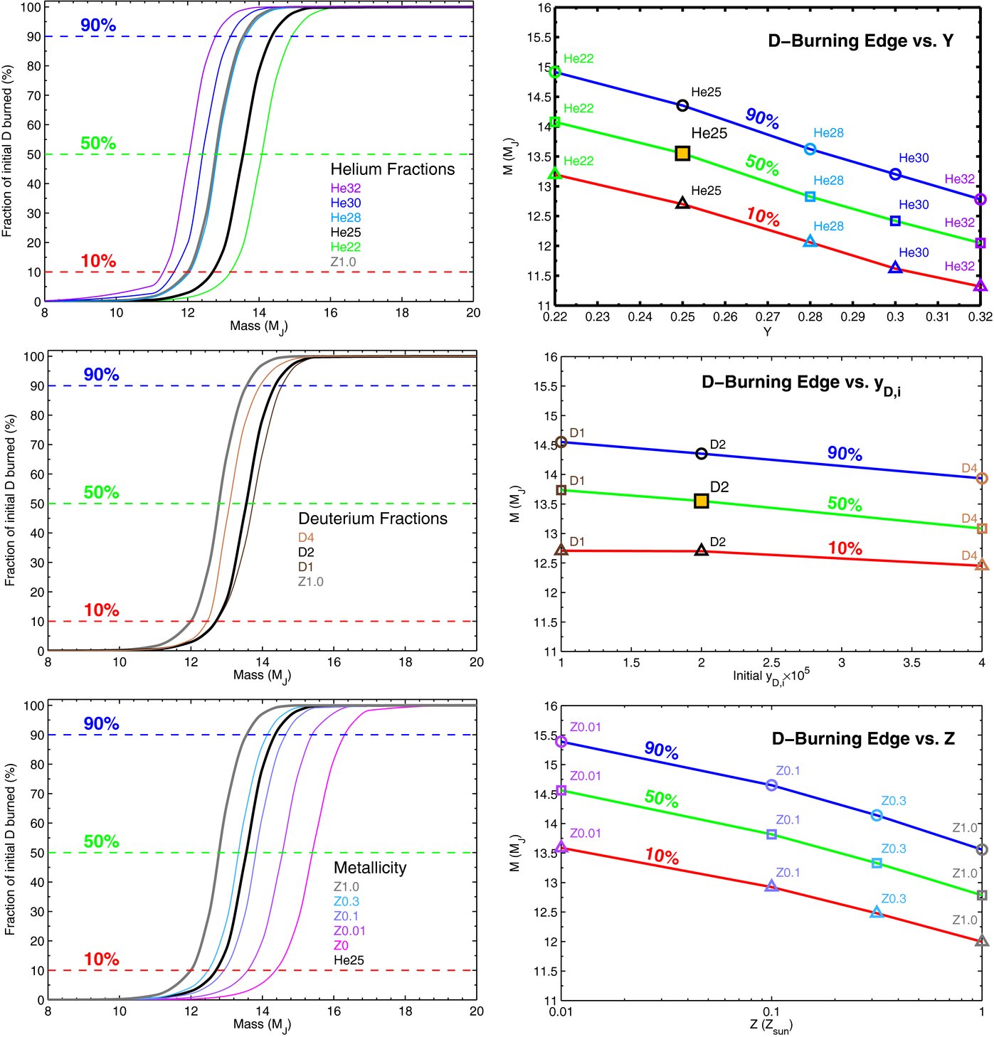
There are four main lessons from the data in Figure 3 and Table 1.

1.
Within each sequence of models, the expected trends hold. That is, greater helium abundance, greater deuterium abundance, and higher metallicity allow a given amount of deuterium to fuse at a lower object mass.
2.
Depending on what is meant by "deuterium burning" (i.e., how much of the initial deuterium must burn to qualify), the deuterium-burning mass limit can vary quite a bit. As the criterion goes from 10% to 50% and from 50% to 90%, the required mass increases by ∼0.8–0.9 M_J.
3.
0.012 M_☉ and 13 M_J is not far from the mass limit for most models.
4.
However, the full range of masses displayed in this table goes from 11.3 M_J (He32, 10%) to 16.3 M_J (Z0, 90%).

With the final point in mind, it is clear that claiming that an object does or does not "burn deuterium" implies a set of physical assumptions about the model and a criterion for deuterium burning. Any criterion is fine, so long as people know what it is; but implicit assumptions should be made explicit, and might not actually apply to some astrophysical objects.

4. DISCUSSION

A useful way to quantify the influence of varying the model parameters on the deuterium mass limit is with the derivative of the mass limit with respect to each model parameter. Although the curves in the right column of Figure 3 do not have constant slope, they are not very far from linear over the ranges shown. In Table 2, we present the average derivative with respect to each parameter. For Y and y_D,i, we take linear derivatives; for y_D,i and Z, we take logarithmic derivatives. These derivatives are not terribly precise measures of the variation, but allow for a quick, crude estimate of the deuterium edge-mass at different parameter values.

Table 2. Approximate Edge-mass Derivatives

Model Sequence	Derivative	Derivative Value
He22–He32	(dM/dY)/100	−0.2 M_J
D1–D4	(dM/dy_D,i)/10⁵	−0.16 M_J
D1–D4	dM/dlog₁₀[y_D,i]	−0.8 M_J
Z0.01–Z1.0	dM/dlog₁₀[Z]	−0.9 M_J
T0.3–T3	dM/dlog₁₀[Z]	−0.7 M_J

Download table as: ASCII Typeset image

Note that, in the calculations discussed so far, the effect of higher metallicity has been reflected only in the atmospheric opacity. In a real object, however, higher metallicity throughout would also lead to an EOS change for the bulk, because high-Z elements have lower electron-to-baryon ratios. As a result, a higher metallicity object would have a higher central density than occurs in our models, and would therefore have a lower deuterium mass limit than we have shown, particularly for model T3. Though there is no published robust EOS that properly includes heavy elements beyond helium, we can approximately correct for this by using a higher helium fraction (this was also done by Guillot 2008). We, therefore, have post-processed our models in an attempt to incorporate this effect. Using values from Asplund et al. (2009), we take Y = 0.2703 and Z = 0.0142 to be the helium and heavy-element mass fractions corresponding to protosolar abundance. Motivated by this, we add 0.0142 in Y for every unit in metallicity (i.e., Y = 0.2703 + 0.0142 for solar, Y = 0.2703 + 2 × 0.0142 for 2× solar, etc.).⁸ We perform a cubic interpolation in Y and use the Z-derivative for model sequence T0.3–T3 to calculate the values in Table 3 corresponding to 0.5, 1, 2, and 3 times solar metallicity. Values of the edge mass in this table then range from ∼11.0 M_J (3× solar, 10% of initial deuterium burned) to ∼13.9 M_J (0.5× solar, 90% of initial deuterium burned).

Table 3. Edge-masses for "Realistic" Treatment of Z

Metallicity	M (10%)	M (50%)	M (90%)
	(M_J)	(M_J)	(M_J)
0.5 × solar^a	12.26	13.10	13.93
1 × solar	11.89	12.73	13.57
2 × solar	11.39	12.23	13.06
3 × solar	10.99	11.83	12.67

Notes. We start with Y = 0.2703 and add 0.0142 in Y for every unit in Z. We perform a cubic interpolation in Y and use the derivatives recorded in the T0.3–T3 row of Table 2 to approximate the combined affects of metallicity on pressure support and on atmospheric opacity. ^aOur adopted value of Z_☉ = 0.0189 is taken from Anders & Grevesse (1989). In absolute units, the quantities in the table correspond to the following values: 0.5 × Z_☉ = 0.00945; 2 × Z_☉ = 0.0378; 3 × Z_☉ = 0.0567.

Download table as: ASCII Typeset image

Although the deuterium-burning mass limits in Tables 1 and 3 vary from 11.0 to 16.3 times Jupiter's mass, a narrower range of values is found if we restrict our attention to a particular burning fraction criterion (50%, say) with realistic Y, y_D,i, and Z values. For helium mass fractions between 0.25 and 0.30, initial deuterium fractions between 10⁻⁵ and 2 × 10⁻⁵, and metallicities between 0.5 and 2 times solar, the mass required to burn 50% of the initial deuterium is between ∼12.2 M_J and ∼13.7 M_J. Values somewhat outside this range are not impossible, but values very far from this range are probably rare.

5. CONCLUSIONS

We have calculated a suite of models of substellar mass objects, encompassing a range of values of helium fraction, initial deuterium fraction, and metallicity. We have also used several calculations of the atmospheric boundary conditions. Although the rate of deuterium burning is extremely sensitive to temperature, it is worthwhile bearing in mind that deuterium will burn at some rate at any nonzero temperature, so one must specify what is meant by "deuterium burning" (i.e., how much of the initial deuterium must burn to qualify). We have found that, depending on what criterion is used, reasonable values for the deuterium mass limit range from ∼11.4 to ∼14.4 times Jupiter's mass; the former limit corresponding to 2× solar metallicity, 10% of initial deuterium burned, and the latter limit to solar metallicity, Y = 0.25%, 90% of initial deuterium burned. Extreme models (very low helium fraction, very low metallicity) could require even higher mass in order to burn a specified percentage of their initial deuterium. The canonical value of 13 M_J (Burrows et al. 1997) is a reasonable estimate of the mass at which significant deuterium burning begins, but this value is model dependent.

Still, one should keep in mind that the deuterium cut is probably less relevant to an object's true taxonomic status than is its formation history. The downside of a "formation scenario" definition is that formation history is not easily observable. On the other hand, though mass might be observable, the parameters Y, y_D,i, and Z might not be. Furthermore, some objects will be found significantly above 13 M_J that will be of clearly "planetary" origin (e.g., CoRoT-3b). Whether to call these objects "brown dwarfs" or "deuterium-burning planets" remains open for debate. Similarly, objects might be found that are significantly less massive than 13 M_J that appear not to have formed in a protoplanetary disk, but rather to be the low-mass end of the brown dwarf formation process. Though classified as "planets" by standard terminology, these objects might be more taxonomically related to brown dwarfs than to planets.

We emphasize that there is really no need at this time to rigidly distinguish between a giant planet and a brown dwarf on the basis of a single criterion. There is ambiguity in the provenance of these objects, and this ambiguity might persist for a while. The use of a particular term ("planet" or "brown dwarf"), should be accompanied by the definition that is employed. Given that planets are thought to be objects in orbit around a star (or around a brown dwarf), while brown dwarfs are thought to be the low-mass end of the star formation process, there is likely to be overlap in the mass range of these objects unless one adopts a rigid mass cut to distinguish them. Doing so, however, will surely lead to an overlap in formation scenarios (as in the case of CoRoT-3b). When classifying a newly discovered substellar-mass object, one can use a variety of "reasonable" criteria, but the classifications should remain tentative until a more thorough observational and theoretical understanding of substellar objects is achieved.

We thank Kevin Heng, Bill Hubbard, Didier Saumon, Jason Nordhaus, and Zimri Yaseen for useful discussions. This study was supported in part by NASA grant NNX07AG80G. We also acknowledge support through JPL/Spitzer Agreements 1328092, 1348668, and 1312647.

THE DEUTERIUM-BURNING MASS LIMIT FOR BROWN DWARFS AND GIANT PLANETS

Article metrics

Permissions

Author e-mails

Author affiliations

Dates

ABSTRACT

1. INTRODUCTION