


ABSTRACT
Recent discoveries of several transiting planets with clearly non-zero eccentricities and some large obliquities started changing the simple picture of close-in planets having circular and well-aligned orbits. The two major scenarios that form such close-in planets are planet migration in a disk and planet–planet interactions combined with tidal dissipation. The former scenario can naturally produce a circular and low-obliquity orbit, while the latter implicitly assumes an initially highly eccentric and possibly high-obliquity orbit, which are then circularized and aligned via tidal dissipation. Most of these close-in planets experience orbital decay all the way to the Roche limit as previous studies showed. We investigate the tidal evolution of transiting planets on eccentric orbits, and find that there are two characteristic evolution paths for them, depending on the relative efficiency of tidal dissipation inside the star and the planet. Our study shows that each of these paths may correspond to migration and scattering scenarios. We further point out that the current observations may be consistent with the scattering scenario, where the circularization of an initially eccentric orbit occurs before the orbital decay primarily due to tidal dissipation in the planet, while the alignment of the stellar spin and orbit normal occurs on a similar timescale to the orbital decay largely due to dissipation in the star. We also find that even when the stellar spin–orbit misalignment is observed to be small at present, some systems could have had a highly misaligned orbit in the past, if their evolution is dominated by tidal dissipation in the star. Finally, we also re-examine the recent claim by Levrard et al. that all orbital and spin parameters, including eccentricity and stellar obliquity, evolve on a similar timescale to orbital decay. This counterintuitive result turns out to have been caused by a typo in their numerical code. Solving the correct set of tidal equations, we find that the eccentricity behaves as expected, with orbits usually circularizing rapidly compared to the orbital decay rate.
Export citation and abstract BibTeX RIS
1. INTRODUCTION
More than 450 exoplanets have been discovered so far. Out of about 360 extrasolar planetary systems, roughly 30% possess close-in planets with semimajor axes a ≲ 0.1 AU. Also, there are 18 out of 45 multiple-planet systems with at least one close-in planet. The mean eccentricity for extrasolar planets with a < 0.1 AU is close to zero, while for planets beyond 0.1 AU, it is e ≃ 0.25. This sharp decline in eccentricity close to the central star is usually explained as a result of efficient eccentricity damping due to tidal interactions between the star and the planet (e.g., Rasio et al. 1996; Jackson et al. 2008). Additionally, there are currently at least 26 systems with measurements of the projected stellar obliquity angle λ (see Table 1) through the Rossiter–McLaughlin (RM) effect (Rossiter 1924; McLaughlin 1924; Ohta et al. 2005; Gaudi & Winn 2007). Although many systems have projected stellar obliquities consistent with zero within 2σ (e.g., Fabrycky & Winn 2009), suggesting near-perfect spin–orbit alignment, there are now several planetary systems that are clearly misaligned (Triaud et al. 2010). Examples include XO-3, HD 80606, and WASP-14, which are in prograde orbits with λ ≃ 37.3 ± 3.7, 53+34−21, and −33.1 ± 7.4 deg, respectively (Winn et al. 2009c, 2009d; Johnson et al. 2009), as well as HAT-P-7, WASP-2, WASP-8, WASP-15, and WASP-17, which have retrograde orbits with λ ≃ 182.5 ± 9.4, −153+15−11, −120 ± 4, −139.6+4.3−5.2, and −147.3+5.5−5.9 deg, respectively (Winn et al. 2009a; Triaud et al. 2010).
Table 1. Data are Taken from http://exoplanet.eu/
| Planet Name | Mp | Rp | a | e | M* | R* | vsin i | λ | Age | References |
|---|---|---|---|---|---|---|---|---|---|---|
| (MJ) | (RJ) | (AU) | (M☉) | (R☉) | (km s−1) | (deg) | (Gyr) | |||
| CoRoT-1 b (G0V) | 1.03+0.12−0.12 | 1.49+0.08−0.08 | 0.0254+0.0004−0.0004 | 0 (fixed) | 0.95+0.15−0.15 | 1.11+0.05−0.05 | 5.2+1.0−1.0 | −77+11−11 | Barge et al. (2008), Pont et al. (2010) | |
| CoRoT-2 b (G7V) | 3.31+0.16−0.16 | 1.465+0.029−0.029 | 0.0281+0.0009−0.0009 | 0 (fixed) | 0.97+0.06−0.06 | 0.902+0.018−0.018 | 11.85+0.50−0.50 | 7.2+4.5−4.5 | ∼0.2–4 | Alonso et al. (2008), Bouchy et al. (2008) |
| CoRoT-3 b (F3V) | 21.23+0.82−0.59 | 0.9934+0.058−0.058 | 0.05694+0.00096−0.00079 | 0.008+0.015−0.005 | 1.359+0.059−0.043 | 1.540+0.083−0.078 | 17.0+1.0−1.0 | −37.6+22.3−10.0 | 1.6–2.8 | Triaud et al. (2009), Deleuil et al. (2008) |
| CoRoT-4 b (F0V) | 0.72+0.08−0.08 | 1.190+0.06−0.05 | 0.09+0.001−0.001 | 0+0.1−0.1 | 1.16+0.03−0.02 | 1.17+0.01−0.03 | 6.4+1.0−1.0 | 1+1.0−0.3 | Moutou et al. (2008) | |
| CoRoT-5 b (F9V) | 0.467+0.047−0.024 | 1.388+0.046−0.047 | 0.04947+0.00026−0.00029 | 0.09+0.09−0.04 | 1.00+0.02−0.02 | 1.186+0.04−0.04 | 1+1−1 | 5.5–8.3 | Rauer et al. (2009) | |
| CoRoT-6 b (F9V) | 2.96+0.34−0.34 | 1.166+0.035−0.035 | 0.0855+0.0015−0.015 | <0.1 | 1.05+0.05−0.05 | 1.025+0.026−0.026 | 7.6+1.0−1.0 | 2.5–3.3 | Fridlund et al. (2010) | |
| CoRoT-7 b (G9V) | 0.0151+0.0025−0.0025 | 0.15+0.008−0.008 | 0.0172+0.00029−0.00029 | 0 | 0.93+0.03−0.03 | 0.87+0.04−0.04 | 1.2–2.3 | Queloz et al. (2009) | ||
| CoRoT-7 c (G9V) | 0.0264+0.0028−0.0028 | 0.046 | 0 | Queloz et al. (2009) | ||||||
| GJ 1214 b (M) | 0.0204 | 0.239 | 0.0143 | <0.27 | 0.157+0.019−0.019 | 0.2110+0.0097−0.0097 | <2.0 | 3–10 | Charbonneau et al. (2009) | |
| GJ 436 b (M2.5) | 0.0729+0.0025−0.0025 | 0.3767+0.0082−0.0092 | 0.02872+0.00029−0.00026 | 0.14+0.01−0.01 | 0.452+0.014−0.012 | 0.464+0.009−0.011 | 0.52+0.05−0.05 | 6.0+4.0−5.0 | TWC08, Levrard et al. (2009) | |
| HAT-P-1 b (G0V) | 0.532+0.030−0.030 | 1.242+0.053−0.053 | 0.0553+0.0012−0.0013 | <0.067 | 1.133+0.075−0.079 | 1.135+0.048−0.048 | 3.75+0.58−0.58 | 3.7+2.1−2.1 | 2.7+2.5−2.0 | TWC08, Johnson et al. (2008) |
| HAT-P-11 b (K4) | 0.081+0.009−0.009 | 0.422+0.014−0.014 | 0.0530+0.0002−0.0008 | 0.198+0.046−0.046 | 0.81+0.02−0.03 | 0.75+0.02−0.02 | 1.5+1.5−1.5 | 6.5+5.9−4.1 | Bakos et al. (2010) | |
| HAT-P-12 b (K4) | 0.211+0.012−0.012 | 0.959+0.029−0.021 | 0.0384+0.0003−0.0003 | 0 | 0.733+0.018−0.018 | 0.701+0.02−0.01 | 0.5+0.4−0.4 | 2.5+2.0−2.0 | Hartman et al. (2009) | |
| HAT-P-13 b (G4) | 0.853+0.029−0.046 | 1.281+0.079−0.079 | 0.0427+0.0006−0.0012 | 0.021+0.009−0.009 | 1.22+0.05−0.10 | 1.56+0.08−0.08 | 2.9+1.0−1.0 | 5.0+2.5−0.7 | Bakos et al. (2009a) | |
| HAT-P-13 c (G4) | 15.2+1.0−1.0 | 1.188+0.018−0.033 | 0.691+0.018−0.018 | Bakos et al. (2009a) | ||||||
| HAT-P-2 b (F8) | 9.09+0.24−0.24 | 1.157+0.073−0.062 | 0.06878+0.00068−0.00068 | 0.5171+0.0033−0.0033 | 1.36+0.04−0.04 | 1.64+0.09−0.08 | 20.8+0.3−0.3 | 1.2+13.4−13.4 | 2.6+0.5−0.5 | Pál et al. (2010), Winn et al. (2007) |
| HAT-P-3 b (K) | 0.596+0.024−0.026 | 0.899+0.043−0.049 | 0.03882+0.00060−0.00077 | 0 | 0.928+0.044−0.054 | 0.833+0.034−0.044 | 0.5+0.5−0.5 | 1.5+5.4−1.4 | TWC08, Torres et al. (2007) | |
| HAT-P-4 b (F) | 0.68+0.04−0.04 | 1.27+0.05−0.05 | 0.0446+0.0012−0.012 | 0 | 1.26+0.06−0.14 | 1.590.07−0.07 | 5.5+0.5−0.5 | 4.2+2.6−0.6 | Kovács et al. (2007) | |
| HAT-P-5 b (G) | 1.06+0.11−0.11 | 1.26+0.05−0.05 | 0.04075+0.00076−0.00076 | 0 | 1.160+0.062−0.062 | 1.167+0.049−0.049 | 2.6+1.5−1.5 | 2.6+1.8−1.8 | Bakos et al. (2007) | |
| HAT-P-6 b (F8) | 1.057+0.119−0.119 | 1.330+0.061−0.061 | 0.05235+0.00087−0.00087 | 0 (fixed) | 1.29+0.06−0.06 | 1.46+0.06−0.06 | 8.7+1.0−1.0 | 2.3+0.5−0.7 | Noyes et al. (2008) | |
| HAT-P-7 b (F6V) | 1.776+0.077−0.049 | 1.363+0.195−0.087 | 0.0377+0.0005−0.0005 | 0 (fixed) | 1.47+0.08−0.05 | 1.84+0.23−0.11 | 3.8+0.5−0.5 | 182.5+9.4−9.4 | 2.2+1.0−1.0 | Pál et al. (2008), Winn et al. (2009a) |
| HAT-P-8 b (F) | 1.52+0.18−0.16 | 1.50+0.08−0.06 | 0.0487+0.0026−0.0026 | 0 (fixed) | 1.28+0.04−0.04 | 1.58+0.08−0.06 | 11.5+0.5−0.5 | 3.4+1.0−1.0 | Latham et al. (2009) | |
| HAT-P-9 b (F) | 0.78+0.09−0.09 | 1.40+0.06−0.06 | 0.053+0.002−0.002 | 0 (fixed) | 1.28+0.13−0.13 | 1.32+0.07−0.07 | 11.9+1.0−1.0 | 1.6+1.8−1.4 | Shporer et al. (2009) | |
| HD 149026 b (G0IV) | 0.359+0.022−0.021 | 0.654+0.060−0.045 | 0.04313+0.00065−0.00056 | 0 | 1.294+0.060−0.050 | 1.368+0.12−0.083 | 6.2+2.1−0.6 | −12+15−15 | 1.9+0.9−0.9 | TWC08, Wolf et al. (2007) |
| HD 17156 b (G0) | 3.22+0.08−0.08 | 1.02+0.08−0.08 | 0.1614+0.0022−0.0022 | 0.6801+0.0019−0.0019 | 1.24+0.03−0.03 | 1.44+0.08−0.08 | 4.18+0.31−0.31 | 10.0+5.1−5.1 | 3.06+0.64−0.76 | Barbieri et al. (2009) Narita et al. (2009), and Winn et al. (2009b) |
| HD 189733 b (K1-2) | 1.138+0.022−0.025 | 1.178+0.016−0.023 | 0.03120+0.00027−0.00037 | 0.0041+0.0025−0.0020 | 0.823+0.022−0.029 | 0.766+0.007−0.013 | 3.316+0.017−0.067 | −0.85+0.32−0.28 | 6.8+5.2−4.4 | Triaud et al. (2009), TWC08 |
| HD 209458 b (G0V) | 0.685+0.015−0.014 | 1.359+0.016−0.019 | 0.04707+0.00046−0.00047 | 0 | 1.119+0.033−0.033 | 1.155+0.014−0.016 | 4.70+0.16−0.16 | −4.4+1.4−1.4 | 3.1+0.8−0.7 | TWC08, Winn et al. (2005) |
| HD 80606 b (G5) | 4.20+0.11−0.11 | 0.974+0.030−0.030 | 0.4614+0.0047−0.0047 | 0.93286+0.00055−0.00055 | 1.05+0.032−0.032 | 0.968+0.028−0.028 | 1.12+0.44−0.22 | 53+34−21 | 1.6+1.8−1.1 | Winn et al. (2009c) |
| Kepler-4 b (G0) | 0.077+0.012−0.012 | 0.357+0.019−0.019 | 0.0456+0.0009−0.0009 | 0 (fixed) | 1.223+0.053−0.091 | 1.487+0.071−0.084 | 2.2+1.0−1.0 | 4.5+1.5−1.5 | Borucki et al. (2010) | |
| Kepler-5 b (?) | 2.114+0.056−0.059 | 1.431+0.041−0.052 | 0.05064+0.00070−0.00070 | <0.024 | 1.374+0.040−0.059 | 1.793+0.043−0.062 | 4.8+1.0−1.0 | 3.0+0.6−0.6 | Koch et al. (2010) | |
| Kepler-6 b (F) | 0.669+0.025−0.030 | 1.323+0.026−0.029 | 0.04567+0.00055−0.00046 | 0 (fixed) | 1.209+0.044−0.038 | 1.391+0.017−0.034 | 3.0+1.0−1.0 | 3.8+1.0−1.0 | Dunham et al. (2010) | |
| Kepler-7 b (F-G) | 0.433+0.040−0.041 | 1.478+0.050−0.051 | 0.06224+0.00109−0.00084 | 0 (fixed) | 1.347+0.072−0.054 | 1.843+0.048−0.066 | 4.2+0.5−0.5 | 3.5+1.0−1.0 | Latham et al. (2010) | |
| Kepler-8 b (F8IV) | 0.603+0.13−0.19 | 1.419+0.056−0.058 | 0.0483+0.0006−0.0012 | 0 (fixed) | 1.213+0.067−0.063 | 1.486+0.053−0.062 | 10.5+0.7−0.7 | −26.9+4.6−4.6 | 3.84+1.5−1.5 | Jenkins et al. (2010) |
| Lupus-TR-3 b (K1V) | 0.81+0.18−0.18 | 0.89+0.07−0.07 | 0.0464+0.0007−0.0007 | 0 (fixed) | 0.87+0.04−0.04 | 0.82+0.05−0.05 | Weldrake et al. (2008) | |||
| OGLE-TR-10 b (G/K) | 0.62+0.14−0.14 | 1.25+0.14−0.12 | 0.0434+0.0013−0.0015 | 0 | 1.14+0.10−0.12 | 1.17+0.13−0.11 | 3+2−2 | 3.2+4.0−3.1 | TWC08, Konacki et al. (2005) | |
| OGLE-TR-111 b (G/K) | 0.55+0.10−0.10 | 1.051+0.057−0.052 | 0.04689+0.0010−0.00097 | 0 | 0.852+0.058−0.052 | 0.831+0.045−0.040 | 8.8+5.2−6.6 | TWC08 | ||
| OGLE-TR-113 b (K) | 1.26+0.16−0.16 | 1.093+0.028−0.019 | 0.02289+0.00016−0.00015 | 0 | 0.779+0.017−0.015 | 0.774+0.020−0.011 | 13.2+0.8−2.4 | TWC08 | ||
| OGLE-TR-132 b (F) | 1.18+0.14−0.13 | 1.20+0.15−0.11 | 0.03035+0.00057−0.00053 | 0 | 1.305+0.075−0.067 | 1.32+0.17−0.12 | 1.2+1.5−1.1 | TWC08 | ||
| OGLE-TR-182 b (G) | 1.01+0.15−0.15 | 1.13+0.24−0.08 | 0.051+0.001−0.001 | 0 | 1.14+0.05−0.05 | 1.14+0.23−0.06 | Pont et al. (2008) | |||
| OGLE-TR-211 b (F7-8) | 1.03+0.20−0.20 | 1.36+0.18−0.09 | 0.051+0.001−0.001 | 0 | 1.33+0.05−0.05 | 1.64+0.21−0.07 | Udalski et al. (2008) | |||
| OGLE-TR-56 b (G) | 1.39+0.18−0.17 | 1.363+0.092−0.090 | 0.02383+0.00046−0.00051 | 0 | 1.228+0.072−0.078 | 1.363+0.089−0.086 | 3 | 3.2+1.0−1.3 | TWC08, Konacki et al. (2003) | |
| TrES-1 (K0V) | 0.752+0.047−0.046 | 1.067+0.022−0.021 | 0.03925+0.00056−0.00060 | 0 | 0.878+0.038−0.040 | 0.807+0.017−0.016 | 1.3+0.3−0.3 | 30+21−21 | 3.7+3.4−2.8 | TWC08, Narita et al. (2007) |
| TrES-2 (G0V) | 1.200+0.051−0.053 | 1.224+0.041−0.041 | 0.03558+0.00070−0.00077 | 0 | 0.983+0.059−0.063 | 1.003+0.033−0.033 | 1.0+0.6−0.6 | −9.0+12.0−12.0 | 5.0+2.7−2.1 | TWC08, Winn et al. (2008) |
| TrES-3 (G) | 1.938+0.062−0.063 | 1.312+0.033−0.041 | 0.02272+0.00017−0.00026 | 0 | 0.915+0.021−0.031 | 0.812+0.014−0.025 | 1.5+1.0−1.0 | 0.6+2.0−0.4 | TWC08 | |
| TrES-4 (F) | 0.920+0.073−0.072 | 1.751+0.064−0.062 | 0.05092+0.00072−0.00069 | 0 | 1.394+0.060−0.056 | 1.816+0.065−0.062 | 8.5+1.2−1.2 | 6.3+4.7−4.7 | 2.9+0.4−0.4 | TWC08, Narita et al. (2010) |
| WASP-1 b (F7V) | 0.918+0.091−0.090 | 1.514+0.052−0.047 | 0.03957+0.00049−0.00048 | 0 | 1.301+0.049−0.047 | 1.517+0.052−0.045 | 5.79+0.35−0.35 | 3.0+0.6−0.6 | TWC08, Stempels et al. (2007) | |
| WASP-10 b (K5) | 2.96+0.22−0.17 | 1.28+0.077−0.091 | 0.0369+0.0012−0.0014 | 0.059+0.014−0.004 | 0.703+0.068−0.080 | 0.775+0.043−0.040 | <6 | 0.8+0.2−0.2 | Christian et al. (2009) | |
| WASP-11 b (K3V) | 0.487+0.018−0.018 | 1.005+0.032−0.027 | 0.0435+0.0006−0.0006 | 0 (fixed) | 0.83+0.03−0.03 | 0.79+0.02−0.02 | 0.5+0.2−0.2 | 7.9+3.8−3.8 | Bakos et al. (2009b) | |
| WASP-12 b (G0) | 1.41+0.10−0.10 | 1.79+0.09−0.09 | 0.0229+0.0008−0.0008 | 0.049+0.015−0.015 | 1.35+0.14−0.14 | 1.57+0.07−0.07 | <2.2+1.5−1.5 | 2+1−1 | Hebb et al. (2009) | |
| WASP-13 b (G1V) | 0.46+0.06−0.05 | 1.21+0.14−0.12 | 0.0527+0.0017−0.0019 | 0 (fixed) | 1.03+0.11−0.09 | 1.34+0.13−0.11 | <4.9 | 8.5+5.5−4.9 | Skillen et al. (2009) | |
| WASP-14 b (F5V) | 7.341+0.508−0.496 | 1.281+0.075−0.082 | 0.036+0.001−0.001 | 0.091+0.003−0.003 | 1.211+0.127−0.122 | 1.306+0.066−0.073 | 4.9+1.0−1.0 | −33.1+7.4−7.4 | ∼0.5–1.0 | Joshi et al. (2009), Johnson et al. (2009) |
| WASP-15 b (F5) | 0.542+0.050−0.050 | 1.428+0.077−0.077 | 0.0499+0.0018−0.0018 | 0 (fixed) | 1.18+0.12−0.12 | 1.477+0.072−0.072 | 4.27+0.26−0.36 | −139.6+4.3−5.2 | 3.9+2.8−1.3 | West et al. (2009), Triaud et al. (2010) |
| WASP-16 b (G3V) | 0.855+0.043−0.076 | 1.008+0.083−0.060 | 0.0421+0.0010−0.0018 | 0 (fixed) | 1.022+0.074−0.129 | 0.946+0.057−0.052 | 3.0+1.0−1.0 | 2.3+5.8−2.2 | Lister et al. (2009) | |
| WASP-17 b (F6) | 0.490+0.059−0.056 | 1.74+0.26−0.23 | 0.0501+0.0017−0.0018 | 0.129+0.106−0.068 | 1.20+0.12−0.12 | 1.38+0.20−0.18 | 10.14+0.58−0.79 | −147.3+5.5−5.9 | 3.0+0.9−2.6 | Anderson et al. (2010), Triaud et al. (2010) |
| WASP-18 b (F9) | 10.30+0.69−0.69 | 1.106+0.072−0.054 | 0.02026+0.00068−0.00068 | 0.0092+0.0028−0.0028 | 1.25+0.13−0.13 | 1.216+0.067−0.054 | 14.67+0.81−0.57 | 5.0+2.8−3.1 | 0.5–1.5 | Hellier et al. (2009a), Triaud et al. (2010) |
| WASP-19 b (G8V) | 1.14+0.07−0.07 | 1.28+0.07−0.07 | 0.0164+0.0005−0.0006 | 0.02+0.02−0.01 | 0.95+0.10−0.10 | 0.93+0.05−0.04 | 4+2−2 | ≳1 | Hebb et al. (2010) | |
| WASP-2 b (K1V) | 0.915+0.090−0.093 | 1.071+0.080−0.083 | 0.03138+0.00130−0.00154 | 0 | 0.89+0.12−0.12 | 0.840+0.062−0.065 | 0.99+0.27−0.32 | −153+15−11 | 5.6+8.4−5.6 | TWC08, Triaud et al. (2010) |
| WASP-3 b (F7V) | 1.76+0.08−0.14 | 1.31+0.07−0.14 | 0.0317+0.0005−0.0010 | 0 | 1.24+0.06−0.11 | 1.31+0.06−0.12 | 13.4+1.5−1.5 | 15+10−9 | 0.7–3.5 | Pollacco et al. (2008), Simpson et al. (2010) |
| WASP-4 b (G7V) | 1.21+0.13−0.08 | 1.304+0.054−0.042 | 0.02255+0.00095−0.00065 | 0 (fixed) | 0.85+0.11−0.07 | 0.873+0.036−0.027 | 2.14+0.38−0.35 | 4+34−43 | 5.2+3.8−3.2 | Gillon et al. (2009b), Triaud et al. (2010) |
| WASP-5 b (G4V) | 1.58+0.13−0.10 | 1.087+0.068−0.071 | 0.0267+0.0012−0.0008 | 0.038+0.026−0.018 | 0.96+0.13−0.09 | 1.029+0.056−0.069 | 3.24+0.34−0.35 | 12.4+8.2−11.9 | 5.4+4.4−4.3 | Gillon et al. (2009b), Triaud et al. (2010) |
| WASP-6 b (G8V) | 0.503+0.019−0.038 | 1.224+0.051−0.052 | 0.0421+0.0008−0.0013 | 0.054+0.018−0.015 | 0.880+0.050−0.080 | 0.870+0.025−0.036 | 1.4+1.0−1.0 | 0.20+0.25−0.32 | 11+7−7 | Gillon et al. (2009a) |
| WASP-7 b (F5V) | 0.96+0.12−0.18 | 0.915+0.046−0.040 | 0.0618+0.0014−0.0033 | 0 (fixed) | 1.28+0.09−0.19 | 1.236+0.059−0.046 | 17+2−2 | Hellier et al. (2009b) | ||
| XO-1 b (G1V) | 0.918+0.081−0.078 | 1.206+0.047−0.042 | 0.04928+0.00089−0.00099 | 0 | 1.027+0.057−0.061 | 0.934+0.037−0.032 | 1.11+0.67−0.67 | 1.0+3.1−0.9 | TWC08, McCullough et al. (2006) | |
| XO-2 b (K0V) | 0.566+0.055−0.055 | 0.983+0.029−0.028 | 0.036840.00040−0.00043 | 0 | 0.974+0.032−0.034 | 0.971+0.027−0.026 | 1.4+0.3−0.3 | 5.8+2.8−2.3 | TWC08, Burke et al. (2007) | |
| XO-3 b (F5V) | 13.25+0.64−0.64 | 1.95+0.16−0.16 | 0.0476+0.0005−0.0005 | 0.260+0.017−0.017 | 1.41+0.03−0.05 | 2.13+0.04−0.05 | 18.54+0.17−0.17 | 37.3+3.7−3.7 | 2.69+0.14−0.16 | Johns-Krull et al. (2008), Winn et al. (2009d) |
| XO-4 b (F5V) | 1.72+0.20−0.20 | 1.34+0.048−0.048 | 0.0555+0.0011−0.0011 | 0 (fixed) | 1.32+0.02−0.02 | 1.56+0.05−0.05 | 8.8+0.5−0.5 | 2.1+0.6−0.6 | McCullough et al. (2008) | |
| XO-5 b (G8V) | 1.059+0.028−0.028 | 1.109+0.050−0.050 | 0.0488+0.0006−0.0006 | 0 | 0.88+0.03−0.03 | 1.08+0.04−0.04 | 0.7+0.5−0.5 | 14.8+2.0−2.0 | Pál et al. (2009) |
Notes. Column (1) planet's name and the stellar spectral type inside the bracket; Column (2) planetary mass; Column (3) planetary radius; Column (4) semimajor axis; Column (5) eccentricity; Column (6) stellar mass; Column (7) stellar radius; Column (8) projected stellar rotational velocity; Column (9) projected stellar obliquity; Column (10) stellar age; Column (11) references, and TWH08 is Torres et al. (2008).
The standard planet formation theory predicts that giant planets are formed beyond the so-called ice line (a ≳ 3 AU), where solid material is abundant due to condensation of ice. To explain the orbital properties of close-in planets, two different scenarios have been proposed. Both of them could potentially explain the proximity of these planets to the stars, but they predict different distributions for orbital inclinations, and possibly eccentricities. One scenario is orbital migration of planets due to gravitational interactions with gas or planetesimal disks (e.g., Goldreich & Tremaine 1980; Ward 1997; Murray et al. 1998), which would naturally bring planets inward from their formation sites. The scenario can also account for the observed small eccentricity and obliquity seen in the majority of close-in planets, because the disks tend to damp eccentricity and inclination of the planetary orbit (e.g., Goldreich & Tremaine 1980; Papaloizou & Larwood 2000). Alternatively, such close-in planets can be formed by tidally circularizing a highly eccentric orbit. A natural way of initially increasing the orbital eccentricity is through gravitational interactions between several planets. Although such interactions alone may not be able to populate the inner region of planetary systems (less than 0.1–1 AU, e.g., Adams & Laughlin 2003; Chatterjee et al. 2008; Matsumura et al. 2010), the orbital eccentricity can be increased due to scattering, ejection, or Kozai cycles (Kozai 1962; Lidov 1962), so that the pericenter of the planetary orbit becomes small enough for tidal interactions with the central star to become important (e.g., Nagasawa et al. 2008). These gravitational interactions also tend to increase the orbital inclination. Chatterjee et al. (2008) performed a number of dynamical simulations of three-planet systems and showed that the final mean inclination of planetary orbits is about 20 deg and that some planets could end up on retrograde orbits (about 2%; S. Chatterjee 2010, private communication). When Kozai cycles increase the orbital eccentricity, the process is called Kozai migration (Wu & Murray 2003). Kozai migration occurring in binary systems may be responsible for at least some of the close-in planets (Fabrycky & Tremaine 2007; Wu et al. 2007; Triaud et al. 2010). One of the goals of our study is to explore the possibility and implications of forming close-in planets via tidal circularization of a highly eccentric planet.
Independent of their formation mechanism, these close-in planets are currently subject to strong tidal interactions with the central star, and such interactions could dominate the orbital evolution of these planets. In multi-planet systems, secular planet–planet interactions may also affect the orbital evolution. However, in Section 2, we will show that it is unlikely that the current and future evolutions of the observed close-in planets are strongly affected by any known or yet-to-be-detected companion (see also Matsumura et al. 2008). In this paper, we investigate tidal evolution of close-in planets to distinguish their two formation scenarios.
Tidal evolution in a two-body system leads to either a stable equilibrium state, or to orbital decay all the way to the Roche limit (Darwin instability; Darwin 1879). Such a study for exoplanetary systems was first done by Rasio et al. (1996), who suggested that 51 Peg b, the only close-in planet known at the time, would be Darwin unstable. In a recent paper, Levrard et al. (2009, hereafter LWC09) investigated the tidal evolution of all transiting planets and pointed out that most of these planets (except HAT-P-2b) are indeed Darwin unstable, and thus undergo continual orbital decay, rather than arriving at a stable, equilibrium orbit (see Section 4.1 and Table 2 for updated results). These Darwin-unstable planets may eventually be accreted by the central star, which has been suggested for some systems observationally (e.g., Gonzalez 1997; Ecuvillon et al. 2006) and numerically (Jackson et al. 2009).
Table 2. Critical Conditions for Tidal Instability, as Well as the Roche Limit for Each System in Table 1
| Planet Name | n/ω* | n/(ω*cos  ) ) |
Prot,* (days) | Ltot/Lc | L*,spin/Lorb | (1/3 − L*,spin/Lorb) | a/aR |
|---|---|---|---|---|---|---|---|
| CoRoT-1 | 7.121 | 31.657 | 10.796 | 0.612 | 0.336 | 1.667 | |
| CoRoT-2 | 2.208 | 2.225 | 3.850 | 0.844 | 0.186 | 2.749 | |
| CoRoT-3 | 0.515 | 0.650 | 2.176 | 1.272 | 0.125 | 0.208 | 13.639 |
| CoRoT-4 | 1.010 | 1.010 | 9.246 | 0.998 | 0.366 | 6.141 | |
| CoRoT-5 | 14.930 | 14.930 | 59.986 | 0.555 | 0.113 | 2.632 | |
| CoRoT-6 | 0.767 | 0.767 | 6.821 | 1.205 | 0.091 | 0.242 | 9.860 |
| CoRoT-7 | 0.000 | 0.000 | 0.000 | 0.149 | 0.000 | 2.764 | |
| GJ1214 | 3.385 | 3.385 | 5.336 | 0.759 | 0.698 | 2.885 | |
| GJ436 | 17.070 | 17.070 | 45.131 | 0.524 | 0.130 | 3.950 | |
| HAT-P-1 | 3.432 | 3.439 | 15.308 | 0.734 | 0.356 | 3.294 | |
| HAT-P-11 | 5.108 | 5.108 | 25.289 | 0.671 | 0.543 | 5.549 | |
| HAT-P-12 | 22.093 | 22.093 | 70.911 | 0.545 | 0.071 | 2.517 | |
| HAT-P-13 | 9.328 | 9.328 | 27.208 | 0.574 | 0.278 | 2.816 | |
| HAT-P-2 | 0.708 | 0.708 | 3.988 | 0.995 | 0.192 | 10.659 | |
| HAT-P-3 | 29.067 | 29.067 | 84.263 | 0.593 | 0.034 | 3.546 | |
| HAT-P-4 | 4.772 | 4.772 | 14.622 | 0.712 | 0.671 | 2.722 | |
| HAT-P-5 | 8.142 | 8.142 | 22.702 | 0.623 | 0.150 | 2.987 | |
| HAT-P-6 | 2.205 | 2.205 | 8.488 | 0.848 | 0.585 | 3.506 | |
| HAT-P-7 | 11.113 | −11.124 | 24.490 | 0.553 | 0.241 | 2.804 | |
| HAT-P-8 | 2.004 | 2.004 | 6.949 | 0.871 | 0.602 | 3.273 | |
| HAT-P-9 | 1.425 | 1.425 | 5.610 | 1.036 | 0.971 | −0.638 | 3.055 |
| HD149026 | 3.881 | 3.968 | 11.160 | 0.868 | 1.270 | 4.094 | |
| HD17156 | 2.286 | 2.294 | 48.555 | 0.945 | 0.025 | 20.702 | |
| HD189733 | 5.269 | 5.270 | 11.684 | 0.722 | 0.113 | 2.809 | |
| HD209458 | 3.526 | 3.537 | 12.429 | 0.731 | 0.379 | 2.799 | |
| HD80606 | 0.392 | 0.651 | 43.714 | 1.054 | 0.011 | 0.323 | 71.577 |
| Kepler-4 | 10.631 | 10.631 | 34.186 | 0.822 | 2.159 | 4.837 | |
| Kepler-5 | 5.325 | 5.325 | 18.893 | 0.671 | 0.208 | 3.889 | |
| Kepler-6 | 7.236 | 7.236 | 23.451 | 0.610 | 0.315 | 2.698 | |
| Kepler-7 | 4.543 | 4.543 | 22.194 | 0.746 | 0.816 | 2.746 | |
| Kepler-8 | 2.034 | 2.281 | 7.158 | 1.021 | 1.273 | −0.939 | 2.567 |
| OGLE-TR-10 | 6.380 | 6.380 | 19.725 | 0.631 | 0.285 | 2.698 | |
| OGLE-TR-111 | 0.000 | 0.000 | 0.000 | 0.632 | 0.000 | 3.670 | |
| OGLE-TR-113 | 0.000 | 0.000 | 0.000 | 0.575 | 0.000 | 2.340 | |
| OGLE-TR-132 | 0.000 | 0.000 | 0.000 | 0.439 | 0.000 | 2.328 | |
| OGLE-TR-56 | 18.964 | 18.964 | 22.979 | 0.489 | 0.207 | 1.734 | |
| TrES-1 | 10.363 | 11.966 | 31.397 | 0.670 | 0.065 | 3.325 | |
| TrES-2 | 20.531 | 20.787 | 50.730 | 0.613 | 0.043 | 2.957 | |
| TrES-3 | 20.960 | 20.960 | 27.380 | 0.622 | 0.039 | 2.117 | |
| TrES-4 | 3.041 | 3.060 | 10.806 | 0.834 | 0.862 | 2.410 | |
| WASP-1 | 5.259 | 5.259 | 13.252 | 0.676 | 0.538 | 2.215 | |
| WASP-10 | 2.120 | 2.120 | 6.533 | 0.988 | 0.068 | 4.431 | |
| WASP-11 | 21.978 | 21.978 | 79.914 | 0.631 | 0.035 | 3.449 | |
| WASP-12 | 33.152 | 33.152 | 36.094 | 0.429 | 0.185 | 1.236 | |
| WASP-13 | 3.178 | 3.178 | 13.832 | 0.779 | 0.619 | 3.169 | |
| WASP-14 | 5.964 | 7.119 | 13.481 | 0.807 | 0.050 | 4.877 | |
| WASP-15 | 4.984 | 4.984 | 18.676 | 0.683 | 0.520 | 2.566 | |
| WASP-16 | 5.113 | 5.113 | 15.949 | 0.695 | 0.161 | 3.746 | |
| WASP-17 | 2.075 | −2.474 | 7.755 | 0.999 | 1.228 | −0.894 | 2.033 |
| WASP-18 | 5.958 | 5.958 | 5.591 | 0.713 | 0.100 | 3.522 | |
| WASP-19 | 14.951 | 14.951 | 11.759 | 0.513 | 0.244 | 1.296 | |
| WASP-2 | 0.000 | 0.000 | 0.000 | 0.578 | 0.000 | 2.815 | |
| WASP-3 | 2.673 | 2.767 | 4.945 | 0.812 | 0.612 | 2.589 | |
| WASP-4 | 16.469 | 16.469 | 22.077 | 0.566 | 0.087 | 1.852 | |
| WASP-5 | 9.151 | 9.151 | 14.870 | 0.614 | 0.134 | 2.760 | |
| WASP-6 | 9.348 | 9.348 | 31.431 | 0.629 | 0.109 | 2.717 | |
| WASP-7 | 0.742 | 0.742 | 3.677 | 1.221 | 0.978 | −0.644 | 5.841 |
| XO-1 | 10.799 | 10.799 | 42.559 | 0.696 | 0.051 | 3.747 | |
| XO-2 | 13.409 | 13.409 | 35.080 | 0.566 | 0.121 | 2.977 | |
| XO-3 | 1.827 | 2.297 | 5.811 | 0.872 | 0.166 | 4.903 | |
| XO-4 | 2.159 | 2.159 | 8.966 | 0.826 | 0.382 | 4.306 | |
| XO-5 | 18.603 | 18.603 | 78.035 | 0.680 | 0.030 | 4.455 |
Download table as: ASCIITypeset image
There is some confusion in the literature concerning the evolution timescales for the various orbital elements. LWC09 studied tidal evolution of transiting planets by taking into account energy dissipation in both the star and the planet. They concluded that all orbital and spin parameters, with the exception of the planetary spin, would evolve on a timescale comparable to the orbital decay timescale. This would imply that both circularity of the orbits and spin–orbit alignment seen in many systems are primordial, because neither obliquity nor eccentricity could be damped to zero before complete spiral-in and destruction of the planet. Unfortunately, after much investigation and comparison with their work, we determined that LWC09 had a typo in their code (confirmed by B. Levrard 2009, private communication), which made them underestimate the energy dissipation inside the planet by several orders of magnitude. By integrating the correct set of tidal evolution equations, we find that there are two characteristic evolutionary paths depending on the relative efficiency of tidal dissipation inside the star and the planet. When the dissipation in the planet dominates, the eccentricity damping time is shorter than the orbital decay time (τe ≪ τa; see Section 4 for details), exactly as expected intuitively (e.g., Rasio et al. 1996; Dobbs-Dixon et al. 2004; Mardling & Lin 2004). On the other hand, when the dissipation in the star dominates, the eccentricity damps on a similar timescale to the orbital decay. We will show that the latter path is fundamentally different from what is suggested by LWC09 in Section 4.2.
There have been many other recent studies of tidal evolution for exoplanets. Jackson et al. (2008) emphasized the importance of solving the coupled evolution equations for eccentricity and semimajor axis. Integrating their tidal evolution equations backward in time, they showed that the "initial" eccentricity distribution of close-in planets matches more closely that of planets on wider orbits; they suggested that gas disk migration is therefore not responsible for all the close-in planets. We reconsider the validity and implication of such a study in Section 5. Barker & Ogilvie (2009) studied the evolution of close-in planets on inclined orbits by including the effect of magnetic braking (Dobbs-Dixon et al. 2004), and pointed out that a true tidal equilibrium state is never reached in reality, since the total angular momentum is not conserved due to magnetized stellar winds. They also showed that neglecting this effect could result in a very different predicted evolution for the systems they considered. Throughout this paper, we compare tidal evolutions with and without the effect of magnetic braking. Another potentially important effect caused by tidal dissipation is the inflation of the planetary radius (Bodenheimer et al. 2001; Gu et al. 2003). Many groups have explored this possibility, motivated by observations of inflated radii for some transiting planets (e.g., Barge et al. 2008; Alonso et al. 2008; Johns-Krull et al. 2008; Gillon et al. 2009b). It appears that at least some of these inflated planets could be explained as a result of past tidal heating (Jackson et al. 2008; Miller et al. 2009; Ibgui & Burrows 2009). More recently, Leconte et al. (2010) revisited this problem and pointed out that the truncated tidal equations used in many previous studies could lead to an erroneous tidal evolution for moderate-to-high eccentricity (e ≳ 0.2). Solving the complete set of tidal equations, they showed that orbital circularization occurs much earlier than previously estimated, and thus only moderately bloated hot Jupiters could be explained as a result of tidal heating. In this paper, we neglect this effect entirely and treat the planetary radius as constant for simplicity (but see Section 5.1).
The outline of the paper is as follows. First, we justify our approach in Section 2 by showing that the current/future evolution of these planets is likely dominated by tidal dissipation, rather than by their gravitational interaction with a more distant object (planet on a wider orbit or distant binary companion). Then, we present our set of tidal evolution equations in Section 3. We re-examine the tidal stability of transiting planets and investigate the tidal evolution forward in time in Section 4. We identify two characteristic evolution paths for Darwin-unstable planets and also discuss the results of LWC09. In Section 5, we explore the past evolution of transiting planets and its implication. Our results imply that each evolutionary path may be consistent with migration and gravitational-interaction-induced formation scenarios of transiting planets, respectively. We also point out that in a limited case, it is possible to have significant stellar obliquity damping before the substantial orbital decay to the Roche limit. In Section 6, we study the different definitions of tidal quality factors and investigate their effects on evolution. Finally, in Section 7, we discuss and summarize our results.
2. POSSIBLE COMPANIONS TO CLOSE-IN PLANETS
In this section, we assess the importance of a known/unknown companion on the current and future evolutions of close-in transiting planets. Secular or resonant interactions with other planets or stellar companions could potentially perturb the planetary orbits significantly. For example, when there is a large mutual inclination between their orbits (≳39 2), Kozai-type (quadrupole) perturbations can become important (Kozai 1962; Lidov 1962). Such highly misaligned systems may naturally occur for binary systems with semimajor axes ≳30–40 AU (Hale 1994), or as a result of planet–planet scattering (Chatterjee et al. 2008; Nagasawa et al. 2008). For smaller mutual inclinations, octupole-level perturbations may still moderately excite the orbital eccentricity, as long as the companion has a non-circular orbit.
For this secular perturbation from a companion to be affecting the current and future evolutions of close-in planets, it must occur faster compared to other perturbations that cause orbital precession. These competing perturbations include general relativistic (GR) precession, tides, as well as rotational distortions (Holman et al. 1997; Sterne 1939). Since the effects of pericenter precession due to stellar and planetary oblateness are usually small compared to those caused by GR precession (Kiseleva et al. 1998; Fabrycky & Tremaine 2007), we simply neglect rotational distortions here.
The pericenter precession timescales corresponding to GR, Kozai-type perturbations (due to a high-inclination perturber), and secular coupling to a low-inclination perturber can be written as follows (Kiseleva et al. 1998; Fabrycky & Tremaine 2007; Zhou & Sun 2003; Takeda et al. 2008):
where the subscripts "*", "p", and "c" indicate the central star, the planet, and the companion body, respectively, while c is the speed of light. In τpp
with the standard Laplace coefficients b(i)3/2(ap/ac) (i = 1, 2). For the secular timescale, the upper sign is chosen when Mp < Mc and the lower one is chosen when Mp>Mc. Such an approximation is reasonable when the system is hierarchical (Takeda et al. 2008) and thus
Following the approach of Matsumura et al. (2008), we compare these various precession timescales to determine which perturbation dominates.
Figure 1 shows the resulting constraints on the mass and orbital radius of the hypothetical planetary/stellar companion for CoRoT-7b and HAT-P-13b. These are the only two known multi-planet systems with a transiting planet, and the companions are shown as the filled circles in the plot. In order to perturb the inner planet significantly despite the GR precession, the companion must exist left of the blue lines to induce Kozai oscillations, and left of the orange line for octupole perturbations to be important. The kink seen in the orange line occurs where Mp ∼ Mc and thus our approximation in calculating the secular timescale breaks down. For HAT-P-13, we find that HAT-P-13c is located left of the blue lines, but right of the orange one. Thus, we expect that HAT-P-13c can perturb the orbit of HAT-P-13b significantly only if they have a large mutual inclination of ≳392. For CoRoT-7, on the other hand, we find that the secular timescale due to CoRoT-7c is comparable to the GR timescale (τpp ∼ τGR). As shown by Ford et al. (2000; see also Adams & Laughlin 2006), such a resonance can increase the eccentricity significantly. However, for small eccentricities e ∼ 0.001, we do not find any significant eccentricity oscillation below a mutual inclination of about 40°. Thus, it is possible that the eccentricity of CoRoT-7b is significantly oscillating if the misalignment of the orbit of CoRoT-7c with respect to CoRoT-7b is large.

Figure 1. Mass and semimajor axis of a hypothetical companion which can affect the orbital evolution of the observed close-in planets in CoRoT-7 and HAT-P-13. The orange line indicates the region within which the secular timescale becomes short compared to the GR timescale. The kink occurs where the approximation for the secular timescale breaks down (see the text). Left and right blue dashed lines indicate similar boundaries for Kozai cycles with the companion eccentricity of 0.2 and 0.9, respectively. Black dotted lines indicate the radial-velocity detection limits for 3, 30, and 100 m s−1. Both of these systems have a known second planet, which is indicated by a filled circle.
Download figure:
Standard image High-resolution imageIn Figure 2, we present similar plots for all transiting planets on an eccentric orbit. The vertical and horizontal lines are drawn for reference at 1 AU and 10 MJ, respectively. It is clear that all systems except HD 80606 are unlikely to have a companion which has a secular perturbation timescale shorter than the GR timescale (left of the orange and blue lines) and at the same time does not cause detectable radial-velocity variations (below the black dotted lines or beyond the observation limit in the semimajor axis). The figure predicts that if a hypothetical planet which can cause a significant secular perturbation is too small to be observed (i.e., a planet exists left of the orange line and below the black dotted lines), its mass would be comparable to Earth or smaller. The figure also predicts that if such a planet cannot be observed now simply because we are not observing long enough (i.e., a planet exists left of the orange line, and beyond, for example, 1 AU), its mass would be comparable to brown dwarfs or larger.
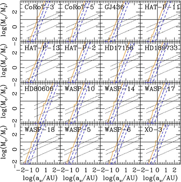
Figure 2. Similar plots to Figure 1 for all transiting planets with an eccentric orbit. Vertical and horizontal lines are drawn at 1 AU and 10 MJ for comparison. It is clear that all systems except HD 80606 are unlikely to have a companion which can cause significant secular perturbations (faster than the GR precession).
Download figure:
Standard image High-resolution imageHD 80606b is in a wide (∼1200 AU) binary system (Eggenberger et al. 2004). However, as can be seen in the figure, this companion cannot induce secular perturbations fast enough compared to the GR precession.
Resonant interactions can work in a similar way, but it is unlikely that all of these planets have such a companion. Thus, the evolution of currently observed transiting planets with an eccentric orbit is likely dominated by tidal dissipation rather than interactions with outer companions.
3. TIDAL EVOLUTION EQUATIONS
In this paper, we numerically study the evolution of observed transiting planets by integrating a set of equations describing the tidal interactions and by assuming that the effect of the known/unknown companions can be neglected.
We follow the general approach of the equilibrium tide model with the weak friction approximation (Darwin 1879). The effects of the dynamical tide are neglected for simplicity. In the absence of any dissipation, the tidally distorted body is assumed to take the equilibrium shape that adjusts itself to the external potential field of the tide-raising body. When the dissipation is non-negligible, the equilibrium surface either lags or leads, depending on whether the spin frequency is smaller or larger than the orbital frequency. In the limit of small viscosities, this phase lag (ϕ) can be approximated to be proportional to the tidal forcing frequency (σ) as ϕ ∼ σΔt. This allows us to interpret the phase lag as the tidal bulge that could have been raised a constant time Δt ago in an inviscid case. Within the context of this model, we can derive the secular equations which are valid for any value of eccentricity and obliquity by following the approach of Alexander (1973) and Hut (1981; also see Leconte et al. 2010). Taking into account tides raised both on the central star by the planet and on the planet by the star, the complete set of tidal equations can be written as follows for the semimajor axis a, eccentricity e, stellar obliquity *, planetary spin ωp, and stellar spin ω*, respectively (e.g., Hut 1981; Levrard et al. 2007). Note that we assume that the planetary obliquity is zero (i.e., the equatorial plane of the planet coincides with the orbital plane). We explicitly write down all equations in order to compare our results with LWC09:
The subscripts "*" and "p" denote the star and planet, respectively. These equations agree with those of Hut (1981) in the limit of small *. In LWC09,  is set to zero (B. Levrard 2009, private communication). This term η is smaller than cos * for most systems, but can be comparable to or larger than cos * for some systems. Examples include CoRoT-1, HD 149026, Kepler-4, Kepler-8, and WASP-17. In the above equations, k2 is the Love number for the second-order harmonic potential (Love 1944), Δt is a constant time lag, n is the mean motion, and α is the square of the radius of gyration with α* = 0.06 and αp = 0.26. The eccentricity functions f1(e2) − f5(e2) are defined as follows as in Hut (1981):
Although it is important to solve the coupled semimajor axis and eccentricity evolution equations (Jackson et al. 2008), the semimajor axis evolution of a planetary system is likely dominated by the energy dissipation in the star. This is because, in an eccentric orbit, a gaseous planet's rotation will be tidally damped to an asymptotic state that is somewhat faster than a value synchronous with the orbital mean motion. The tidal torque is strongest at pericenter where the orbital angular velocity exceeds the orbital mean motion, and therefore the tidal torque averaged around the orbit vanishes when the rotation rate exceeds the mean motion n. This asymptotic state is often referred to as pseudosynchronous rotation. When the planetary spin period and the orbital period approach pseudosynchronization ωp ∼ n, the contribution from the second term in Equation (7) becomes negligible for planets with small eccentricities. Therefore, unless the eccentricity is very high, the orbital evolution is largely determined by the tidal dissipation in the star.
It is not immediately clear whether the tidal energy dissipation leads to either orbital decay or orbital expansion. For all transiting systems except CoRoT-3, CoRoT-6, HAT-P-2, HD 80606, and WASP-7, the host star rotates slowly compared to the orbit (i.e., ω* < n, see Table 2). Therefore, the tidal dissipation in the star tends to lead to orbital decay by transferring angular momentum from the orbit to the stellar spin. On the other hand, when the host star is rapidly spinning, planets could migrate outward, which may have prolonged the lifetime of some of the exoplanets (Dobbs-Dixon et al. 2004). In Section 4.1, we show that HAT-P-2 is Darwin unstable and migrating inward, while the other systems with a rapidly rotating host star are evolving toward the stable tidal equilibria. More specifically, CoRoT-3, CoRoT-6, and WASP-7 are currently migrating outward toward the stable tidal equilibria, while HD 80606 is migrating inward toward the stable state.
By comparing Equations (7) and (8), we see that the eccentricity may be damped on a similar timescale to the semimajor axis, when the eccentricity damping is dominated by the tidal dissipation in the star (i.e., the first term in Equation (8) is much larger than the second term). We discuss this further in the following section.
In some of our calculations, we also take into account the stellar magnetic braking effects, and thus the loss of angular momentum due to stellar winds. For this purpose, we assume that Skumanich's law describes the decrease of the stellar spin sufficiently well so that the average surface rotation velocities of stars that are not interacting with close-in planets can be related to the stellar age (τage) as  (Skumanich 1972). From this relation, the change in the stellar spin can be written as follows:
where γ is a calibration factor and the subscript "0" denotes the normalization factors. By choosing V*,0 = 4 km s−1 and τage, 0 = 1 Gyr as in Dobbs-Dixon et al. (2004), we can define β ≡ γ1.5 × 10⁻¹⁴ yr. We adopt γ = 0.1 for F stars and γ = 1 for G, K, and M stars as in Barker & Ogilvie (2009). For F stars, the smaller calibration factor is chosen since magnetic braking is less efficient due to the very thin or completely absent outer convective layer. We add −β ω3* to Equation (11) when including the effects of magnetic braking.
3.1. Tidal Quality Factors
It is common to describe the dissipation inefficiency of tides in terms of the tidal quality factor instead of a constant lag angle ϕ, or a constant time lag Δt. The specific dissipation function is defined as follows (Goldreich 1963):
where E* in the numerator is the peak energy stored in tides during one tidal cycle, while the denominator represents the energy dissipated over the cycle. When the phase angle ϕ (which is twice the geometrical lag angle) is small, this is simplified as Q ∼ 1/ϕ, which implies a large Q value. The estimated tidal quality factors are ≳104 for Jupiter and Neptune (e.g., Lainey et al. 2009; Zhang & Hamilton 2008), and even larger values are expected for synchronized close-in exoplanets (Ogilvie & Lin 2004). On the other hand, the values usually adopted are ≳106 for main-sequence stars (e.g., Trilling et al. 1998). Thus, we are generally interested in the case of Q ≫ 1, and the above approximation is reasonable. Using the weak friction approximation (ϕ ∼ σΔt), we can redefine Q as
In the following sections, we study some limiting cases of tidal frequencies. Before the spin–orbit synchronization, the tidal dissipation is generally dominated by the semidiurnal tide with the forcing frequency of σ = |2ω − 2n| (Ferraz-Mello et al. 2008). In this case, the tidal quality factor can be written as
As the system approaches synchronization, the effect due to the semidiurnal tide diminishes, and the annual tide with σ = |2ω − n| prevails (Ferraz-Mello et al. 2008). The corresponding tidal quality factor can be written in a similar manner to the above as
Note that when ω = n, the most efficient energy dissipation occurs on the same timescale as the orbital period.
In Sections 4 and 5, we rewrite Equations (7)–(11) by assuming that both stellar and planetary tidal quality factors change as Q ∝ 1/n, while in Section 6, we adopt Q* ∝ 1/|2ω − 2n| and Qp ∝ 1/|2ω − n|. The former is chosen to compare our results with the study of LWC09. For the latter, we are implicitly assuming that close-in exoplanets are pseudosynchronized, while their host stars are not. We will see that this is a reasonable approximation in Section 4.
Throughout this paper, we discuss our results in terms of the modified tidal quality factor Q' ≡ 1.5Q/k2, where k2 is the Love number for the second-order harmonic potential (Love 1944).
4. FUTURE TIDAL EVOLUTION OF TRANSITING PLANETS
4.1. Two Evolutionary Paths for Darwin-unstable Extrasolar Planets
In this section, we revisit the tidal stability problem for transiting extrasolar planets and show that there are two distinct evolutionary paths for Darwin-unstable systems. Throughout this section, we assume that the total angular momentum is conserved (i.e., magnetic braking is neglected). We take into account the magnetic braking effects later in Section 4.3.
The existence and stability of tidal equilibrium states were investigated by many authors (e.g., Hut 1980; Peale 1986; Chandrasekhar 1987; Lai et al. 1994) for binary systems and the solar system. Minimizing the total energy under the constraint of conservation of the total angular momentum, Hut (1980) found that all equilibrium states are characterized by orbital circularity, spin–orbit alignment, and synchronization of the stellar rotation with the orbit. He also showed that equilibrium states exist only when the total angular momentum of the system Ltot is larger than some critical value Lcrit, and that such equilibrium states are unstable when the orbital angular momentum is less than three times the total spin angular momentum (Lspin/Lorb>1/3). In this paper, we are interested in the ultimate fate of close-in exoplanets, and thus we call a system "Darwin stable" only when it is expected to evolve ultimately toward a stable equilibrium state. All other systems are called "Darwin unstable."
First, we check whether the stable tidal equilibrium states exist for the currently known transiting planets listed in Table 1. Tidal equilibrium can only exist when both primary and secondary, with zero obliquities, are synchronously rotating with their orbital motion. Under these constraints, the total angular momentum

has a minimum as a function of the semimajor axis a when Lorb = 3Lspin and
Here, C = αMR2 is the moment of inertia and  is the orbital angular momentum. For Ltot < Lcrit, there can be no tidal equilibrium; for Ltot>Lcrit, two equilibrium states exist. The inner state (Lorb < 3Lspin) is unstable, so the only stable tidal equilibrium is the outer state, which requires Lorb>3Lspin (e.g., Hut 1980; Peale 1986; also see the top panel of Figure 3). A local example of dual synchronous rotation is the Pluto–Charon system (e.g., Peale 1986).
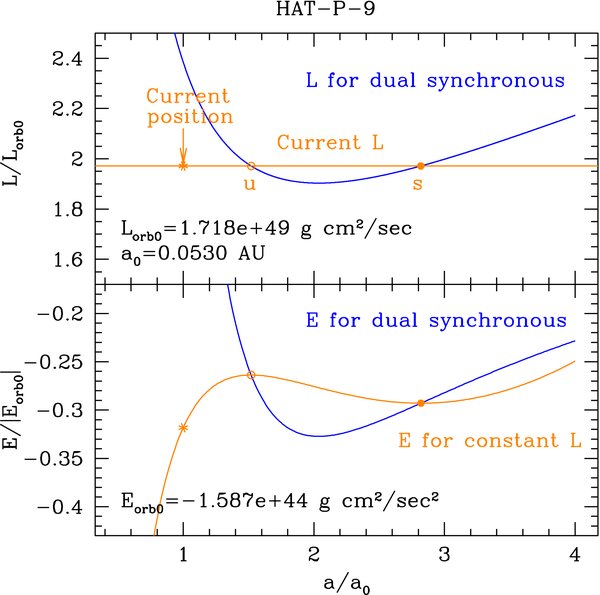
Figure 3. Tidal equilibrium curves as a function of orbital separation for HAT-P-9. The total angular momentum and total energy for dual synchronous states are plotted in blue curves, while the corresponding curves with the constant angular momentum are plotted in orange. The current values are indicated by a star, while open and filled circles with u and s denote unstable and stable tidal equilibria, respectively. Although HAT-P-9 has tidal equilibria, the system currently exists inside the unstable tidal equilibrium state. Therefore, HAT-P-9 is Darwin unstable and migrates toward the central star as the energy dissipates.
Download figure:
Standard image High-resolution imageThe results are summarized in Table 2. As already pointed out by LWC09, most systems have no tidal equilibrium states (i.e., Ltot/Lcrit < 1), and thus are Darwin unstable (i.e., the planet will eventually fall all the way to the Roche limit of the central star, even when the total angular momentum is strictly conserved). Note that, using the refined parameters in Pál et al. (2010), even HAT-P-2, which was the only system with tidal equilibria in LWC09, in fact now appears to have no such states (Ltot/Lcrit = 0.995).
There are several systems which have tidal equilibria (Ltot/Lcrit ≳ 1), and thus could be Darwin stable, namely, CoRoT-3, CoRoT-6, HAT-P-9, HD 80606, Kepler-8, WASP-7, and WASP-17. Among these, CoRoT-3, CoRoT-6, and HD 80606 are clearly evolving toward the stable equilibrium state, since they all have L*,spin/Lorb < 1/3. Therefore, these systems are Darwin stable. Out of the systems with L*,spin/Lorb>1/3, WASP-17 is Darwin unstable, independent of the 1/3 criterion, since it is in a retrograde orbit (Lorb < 0) and thus has Lspin>Lorb. For the other systems (HAT-P-9, Kepler-8, and WASP-7), we checked their tidal equilibrium states as in Figure 3. Here, we compare the total angular momentum and total energy for the dual synchronous state with the current values. As clearly seen in the figure, HAT-P-9 is Darwin unstable, since the system is inside the inner unstable equilibrium state. Most of the angular momentum in the system is in the spin, and the planet falls toward the central star as a result of tidal energy dissipation. Similarly, Kepler-8 is Darwin unstable since the system is far inside the inner unstable equilibrium state. On the other hand, WASP-7 exists just outside the inner unstable equilibrium state, and thus is migrating outward, toward the stable tidal equilibrium state. Similar plots for CoRoT-3, CoRoT-6, and HD 80606 reveal that CoRoT-3 and CoRoT-6 are migrating outward toward the stable equilibria, while HD 80606 is migrating inward toward the stable state. For systems with non-zero eccentricities (CoRoT-3, HD 80606, and WASP-17), we show the evolution explicitly in Figure 6. In short, we find that all planetary systems in Table 1 except CoRoT-3, CoRoT-6, HD 80606, and WASP-7 are Darwin unstable.
The rest of the transiting systems have no tidal equilibrium (Ltot/Lcrit < 1) with the fiducial orbital and spin parameters listed in Table 1, and thus should be Darwin unstable. However, some of them are borderline systems with Ltot/Lcrit ≃ 1, and they could be either Darwin stable or unstable within the observational uncertainties or depending on the value of the unknown parameters (e.g., stellar obliquity). As an example, we show the tidal evolution of a hypothetical planet with Mp = 3MJ and Rp = 1.2RJ orbiting a Sun-like star. We assume the initial semimajor axis, eccentricity, and stellar velocity of a = 0.06 AU, e = 0.3, and v* = 10 km s−1. Such a system would have a stable tidal equilibrium if the stellar obliquity is small, because Ltot/Lcrit ∼ 1.040 and L*,spin/Lorb ∼ 0.193 < 1/3. In Figure 4, we show the results of tidal evolution for two different stellar obliquities of * = 20° and 60°. Here the tidal quality factors are scaled as Q' = Q'0n0/n, where 0 indicates the initial/current values. This scaling ensures that our model is consistent with the constant time lag model as shown in Section 3.1. For each obliquity, we performed three different runs with the same Q'*,0 = 106 and different Q'p,0 of 105, 106, and 107. For the smaller stellar obliquity (* = 20°), we find that the system arrives at the stable tidal equilibrium as circularization, synchronization, and alignment are achieved. On the other hand, for the larger stellar obliquity (* = 60°), the system turns out to be Darwin unstable, and the planet spirals into the star on a ∼10 Gyr timescale. The examples of these borderline systems include HAT-P-2, WASP-10, and XO-3. XO-3 was a Darwin-stable system with previously obtained observed parameters, while HAT-P-2 and WASP-10 can be Darwin stable within the uncertainties as we see in Figure 6.
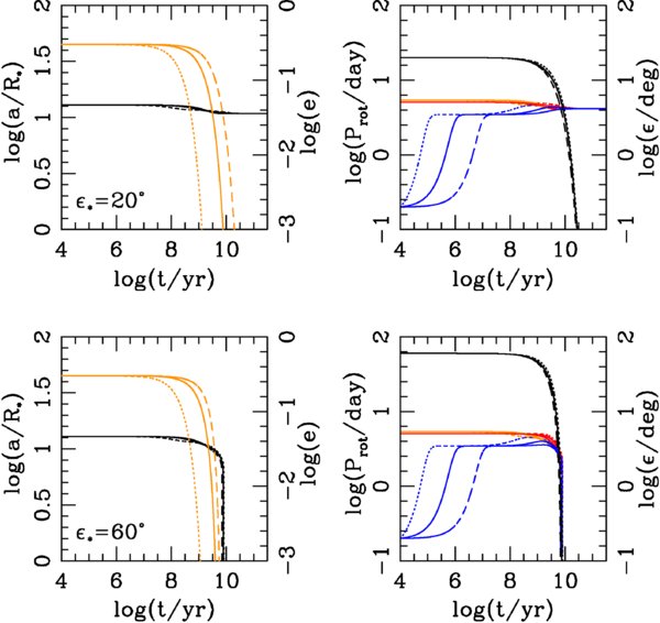
Figure 4. Tidal evolution of a planet with 3 MJ at 0.06 AU and e = 0.3. In the left panels, the black and orange curves show the evolution of the semimajor axis and eccentricity, respectively. In the right panels, the orange curves show the evolution of orbital period, while the blue and red curves show that of planetary and stellar spin periods, respectively. The black curves indicate the evolution of stellar obliquity. The dotted, solid, and dashed curves correspond to cases with the same Q'*,0 = 106 and different Q'p,0 of 105, 106, and 107, respectively. Top panels show the cases with * = 20°, which are Darwin stable, and bottom panels show the cases with * = 60°, which are Darwin unstable.
Download figure:
Standard image High-resolution imageThe tidal evolution is not completely simple even for clearly Darwin-unstable systems. The bottom panels of Figure 4 demonstrate that such systems can take either of two different evolutionary paths, depending on the relative efficiency of tidal dissipation inside the star and the planet. With the smaller planetary tidal quality factors and thus with a more efficient tidal dissipation in the planet (Q'p,0 = 105 and 106 in the figure, which correspond to the dotted and solid curves, respectively), the planetary orbit circularizes before the planet spirals into the Roche limit (τe < τa), while with the larger planetary tidal quality factors (Q'p,0 = 107 in the figure, corresponding to the dashed curves), the circularization time becomes comparable to the orbital decay time (τe ∼ τa). The difference occurs because the orbital decay time is largely determined by the dissipation inside the star, while the circularization time can be determined by either the dissipation inside the star, or that inside the planet. This is apparent from the figure—the orbital decay times are similar for different Q'p,0 values, which means that the semimajor axis evolution is largely independent of the tidal dissipation in the planet and instead is determined entirely by the dissipation in the star (τa ∼ τa,*). On the other hand, the eccentricity damping timescales change significantly for different Q'p,0 values, which suggests that the dissipation in the planet plays a significant role in circularization. However, the circularization time is never longer than the orbital decay time. Therefore, when the expected circularization time from Q'p is longer than the orbital decay time, the eccentricity damping time is also determined by the stellar tidal dissipation (τe ∼ τe,*, which corresponds to Q'p,0 = 107 case in the figure). We show that these results are generally true in Section 4.3.
Unfortunately, it is nontrivial to constrain tidal quality factors and determine which type of evolution each system would follow. This is because tidal quality factors depend sensitively on the detailed interior structure of the body (either star or planet), as well as the tidal forcing frequency and amplitude, and are unlikely to be expressed as a simple constant value (e.g., Ogilvie & Lin 2004, 2007; Wu 2005). However, since we observe a sharp eccentricity decline within a ≲ 0.1 AU, and many Darwin-unstable extrasolar planets are observed to be on nearly circular orbits, it is likely that the eccentricity damping time tends to be short compared to the orbital decay time (τe < τa). We discuss this issue further in Section 5.2.
In summary, we find that there are two evolutionary paths for Darwin-unstable planets—the "stellar-dissipation-dominated" case in which all the parameters except planetary spin evolve on a similar timescale ( ), and the "planetary-dissipation-dominated" case in which circularization occurs before any significant orbital decay (
 ). In the former case, not only the evolution of stellar spin and obliquity, but also that of the semimajor axis and eccentricity, are controlled by the efficiency of tidal dissipation in the star. In the latter case, eccentricity damping is driven by the dissipation in the planet, while orbital decay is largely determined by the dissipation in the star.
4.2. Comparison with Levrard et al. (2009)
Note that, although the stellar-dissipation-driven case (τe ∼ τa) looks similar to the one illustrated by LWC09, there are fundamental differences. In Figure 2 of LWC09, the exponential eccentricity damping approximation, in which they only integrate the planetary dissipation term in the eccentricity evolution, shows a faster damping time than the tidal evolution involving both stellar and planetary energy dissipation. Generally, however, this approximation should provide a timescale comparable to, or longer than, what is obtained with the full integration. This is because most planet-hosting stars are spinning slower than the orbital frequency (see Table 2), and thus energy dissipation in the star accelerates the eccentricity damping, rather than slowing it down (see also Dobbs-Dixon et al. 2004). Therefore, for most systems, the exponential damping approximation involving only the dissipation in the planet should provide an upper limit for eccentricity damping.
We demonstrate this in Figure 5 by taking HD 209458 (the same system considered in LWC09) as an example. Note however that, with current data, HD 209458 has an orbital eccentricity consistent with zero, and thus is not included in the analysis presented in the rest of this paper. We adopt the same initial conditions and assumptions and use the same set of tidal equations as LWC09. Here, the tidal quality factors are initially Q'p,0 = Q'*,0 = 106 and scale as Q' = Q'0n0/n. Our result is shown in the top panel of Figure 5. We find that the tidal evolution in Figure 2 of LWC09 is recovered except for the eccentricity. In our results, the eccentricity evolves on a timescale consistent with the exponential eccentricity damping approximation (dashed line, which is completely overlapped with solid line in the top left panel). In other words, the eccentricity damps on the timescale determined by the tidal dissipation in the planet, as previously shown by many authors (e.g., Rasio et al. 1996; Dobbs-Dixon et al. 2004; Mardling & Lin 2004). For the middle panels, we assume a less efficient tidal dissipation for the planet (Q'p,0 = 109). In this case, we obtain an eccentricity evolution similar to LWC09, but the planetary spin–orbit synchronization, as expected, occurs more slowly. Note that the dashed curve is the eccentricity damping approximation with Q'p,0 = 106. Finally, for the bottom panels, we reproduce Figure 2 of LWC09 by artificially reducing the planetary contribution term in the eccentricity evolution equation (i.e., the second term in Equation (8)), by a factor of 103, i.e., completely suppressing the eccentricity damping effect due to the planet.5 As already mentioned, this discrepancy occurs because the numerical results in LWC09 indeed underestimated the eccentricity damping in the planet, since their code incorrectly had an additional factor of n multiplied in the second term of Equation (8) (B. Levrard 2009, private communication).

Figure 5. Evolution of the orbital and spin parameters of HD 209458 (cf. Figure 2 of LWC09). Three different cases are shown from top to bottom. In all cases, the integrations are stopped when the planet formally hits the stellar surface. In the left panels, the black and orange curves represent the evolution of the semimajor axis and eccentricity, respectively. The dashed orange curve is the exponential damping approximation. In the right panels, the black, blue, and red curves show the evolution of stellar obliquity, planetary, and stellar spins, respectively. In the top panels, we assume the same initial conditions as LWC09, with Q'p,0 = Q'*,0 = 106. The evolution for all parameters but eccentricity looks similar to LWC09's results. The eccentricity evolution follows the exponential damping approximation. In the middle panels, we use the same initial conditions as in the top panels, but assume a less efficient tidal damping in the planet (Q'p,0 = 109). In this case, the eccentricity evolution resembles the one in LWC09, but the planetary spin–orbit synchronization occurs on a longer timescale, as expected. In the bottom panels, we use the same initial conditions as in the top panels, but artificially multiply the eccentricity evolution contribution from the planet by some small factor. Here, we recover the results of LWC09.
Download figure:
Standard image High-resolution image4.3. Lifetimes of Transiting Planets on Eccentric Orbits
In Section 4.1, we identify two characteristic evolutionary paths for Darwin-unstable planets. We now study the tidal evolution of eccentric transiting planets by integrating the tidal equations forward in time with various tidal quality factors, and further investigate the implications of these two paths.
We use the currently observed parameters as initial conditions (see Table 1). The orbital and stellar spin parameters are taken from The Extrasolar Planets Encyclopedia (http://exoplanet.eu/) and references therein. For the planetary spin period, we assume a small initial value (0.2 days), but the overall results are not affected by the exact choice of this value. This is because the planetary spin carries a very small angular momentum, and thus pseudosynchronization with the orbit is achieved very quickly (see also LWC09). For the stellar obliquity, we use the observed projected value λ when RM measurements are available. Here, we implicitly assume that both the angle between the stellar spin axis and the line of sight (i*) and the angle between the orbital angular momentum and the line of sight (i0) are ≃90°. Thus, from cos * = sin i*cos λsin i0 + cos i*cos i0 (Fabrycky & Winn 2009), the stellar obliquity becomes comparable to the projected one (* ≃ λ). For systems without RM measurements, we assume an initial stellar obliquity *,0 = 2°. This choice is rather arbitrary, but is motivated by the typical projected obliquity observed (see Table 2).
First, we show the tidal evolution for typical tidal quality factors (Q'*,0 = Q'p,0 = 106), with the scaling of Q' = Q'0n0/n, and without magnetic braking effect. Our goal here is to show how different the evolution can be within observational uncertainties. We exclude WASP-12 and HAT-P-1 from our analysis because of the uncertainty in their age. The evolution of the semimajor axis and eccentricity of each system is shown in Figure 6. In each panel, we show the results of five different integrations. The solid curves represent the results with fiducial values of a and e, while the dotted curves correspond to four different combinations of maximum and minimum a and e values within their error bars. As expected from Section 4.1, the Darwin-stable systems CoRoT-3 and HD 80606 migrate outward and inward, respectively, and arrive at their tidal equilibrium, with orbital decay eventually stopping. The borderline systems HAT-P-2 and WASP-10 are likely Darwin unstable, but may arrive at a stable tidal equilibrium within the observed uncertainties. Thus, it is important to know the orbital and spin parameters as well as possible to determine the final fate of these borderline systems. The other systems are definitely Darwin unstable within the current observational accuracy, and their planets spiral toward the central star on different timescales. The vertical lines indicate the estimated ages with uncertainties. With Q'*,0 = Q'p,0 = 106 some systems undergo orbital decay too quickly to be compatible with their likely age (e.g., WASP-18, XO-3). Therefore, these results clearly imply that a single set of values for the tidal quality factors cannot reasonably apply to all systems (also see, for example, Matsumura et al. 2008).

Figure 6. Evolution of the semimajor axis (black curves) and eccentricity (orange curves) for Q'*,0 = Q'p,0 = 106. Tidal quality factors scale as Q' = Q'0n0/n, and magnetic braking is not included. The solid curves correspond to the fiducial values, while the dotted curves correspond to four different combinations of maximum and minimum semimajor axis and eccentricity, allowed within the uncertainties. The vertical lines show the age of each system (dashed lines) with uncertainties (dotted lines). As expected from Section 4.1, CoRoT-3 and HD 80606 arrive at their stable tidal equilibrium, while the other planets spiral into the central star. This figure clearly demonstrates that different tidal quality factors apply to different systems, since some planets fall within the Roche limit of their stars on timescales much shorter than the age of the star with a common value of Q'*,0.
Download figure:
Standard image High-resolution imageWe repeated the above calculations for various initial stellar and planetary tidal quality factors ranging over the interval 104 ⩽ Q'0 ⩽ 109, with the scaling of Q' = Q'0n0/n. In Figure 7, we show the range of values for the tidal quality factors that allow planets to survive (a ≳ R*) and stay eccentric (e ≳ 0.001) for 0.1, 1, and 10 Gyr. Here, magnetic braking is not included. For Darwin-stable systems (CoRoT-3 and HD 80606 in our list), the minimum stellar and planetary tidal quality factors correspond to the orbital circularization times. For all Darwin-unstable transiting systems with non-circular orbits, we find the same trend as in Section 4.1: the circularization time is largely determined by the dissipation in the planet, while the survival time is largely determined by the dissipation inside the star. In other words, for Darwin-unstable planets, the minimum planetary tidal quality factors can be inferred from the circularization time, while the minimum stellar tidal quality factors can be inferred from the orbital decay time. We demonstrate this below.
The approximate minimum planetary tidal quality factor that allows a planet to keep a non-circular orbit (e ≳ 0.001) for a certain time (in our examples, 0.1–10 Gyr) can be determined by assuming that the eccentricity evolution depends only on the tidal dissipation inside the planet (de/dt) ≃ (de/dt)p. We rewrite Equation (8) as follows by assuming pseudosynchronization of the planetary spin (dωp/dt = 0), as well as conservation of angular momentum (a(1 − e2) = const):
By integrating the above equation from the currently observed eccentricity to e = 0.001, and solving for Q'p,0, we obtain the minimum planetary tidal quality factors to keep a non-circular orbit for 0.1, 1, and 10 Gyr. These values are plotted as the vertical dashed lines in Figure 7.

Figure 7. Combinations of stellar and planetary tidal quality factors which keep a non-zero eccentricity and allow survival of the planet in forward integration of the tidal equations for 0.1, 1, and 10 Gyr (orange, green, and blue regions, respectively). Magnetic braking is not included, and tidal quality factors change as Q' = Q'0n0/n. The vertical and horizontal dashed lines are determined by assuming (de/dt) ∼ (de/dt)p and (da/dt) ∼ (da/dt)*, respectively (see the text for details). The system's lifetime is largely determined by the tidal dissipation in the star and the circularization by that in the planet.
Download figure:
Standard image High-resolution imageSimilarly, we can determine the approximate minimum stellar tidal quality factor that allows a planet to survive for a certain time before plunging into the central star by assuming that the semimajor axis evolution depends only on the tidal dissipation inside the star (da/dt) ≃ (da/dt)*. Note that this is a reasonable approximation when the pseudosynchronization of the planetary spin is achieved, and the orbit is nearly circular. By setting e = 0, we rewrite Equation (7) as follows:
We integrate the above equation from a = a0(1 − e20) to R* and solve for Q'*,0 to obtain the horizontal dashed lines. Here, we make use of the fact that the difference in eccentricity damping times does not strongly affect the orbital decay time and assume that the orbital decay time of any eccentric Darwin-unstable system can be well described by that of a system with equal angular momentum and a circular orbit.
As seen in Figure 7, the agreement of both the horizontal and vertical dashed lines with the calculations for Darwin-unstable systems is very good. Since Darwin-stable systems (CoRoT-3 and HD 80606) arrive at the stable tidal equilibria and stop migrating, the horizontal dashed lines for these systems significantly differ from the calculated results. Now we present some example runs along the horizontal and vertical lines for WASP-17 to better understand their implications. The left panel of Figure 8 shows three runs along the lowermost horizontal line that corresponds to the survival time of 0.1 Gyr. The dotted, solid, and dashed curves show the evolutions with the same initial stellar tidal quality factor Q'*,0 = 9.13 × 10⁴, and different initial planetary tidal quality factors Q'p,0 = 7.43 × 10⁴, 7.43 × 10⁵, and 7.43 × 10⁶, respectively. The figure confirms that the orbital decay time is largely determined by the tidal dissipation in the star, since there is no obvious difference depending on Q'p,0 values. At the vertex of the vertical and horizontal dashed lines in Figure 7 (i.e., (Q'*,0, Q'p,0) = (9.13 × 10⁴, 7.43 × 10⁵)), we find that the semimajor axis and eccentricity damp roughly on the similar timescale (τe ∼ τa ∼ 0.1 Gyr). For the smaller Q'p,0, the eccentricity damps much faster than the orbital decay (τe < τa ∼ 0.1 Gyr), while for the larger Q'p,0, the eccentricity damps slower than expected from the other two curves and on a similar timescale to the orbital decay (τe ∼ τa ∼ 0.1 Gyr). Similarly, the right panel of Figure 8 shows three runs with the same initial planetary tidal quality factor Q'p,0 = 7.43 × 10⁵ and different initial stellar tidal quality factors Q'*,0 = 9.13 × 10³, 9.13 × 10⁴, and 9.13 × 10⁵. When Q'*,0 is smaller than the vertex value, the orbit decays much faster than 0.1 Gyr, and the circularization occurs on the similar timescale (τe ∼ τa < 0.1 Gyr). On the other hand, when Q'*,0 is larger than the vertex value, the orbit decays much slower than 0.1 Gyr, and the circularization time is shorter than the orbital decay time (τe ∼ 0.1 Gyr < τa). The figure also implies that the orbital circularization time is largely determined by the dissipation in the planet unless τe ∼ τa. Thus, we find that τe ∼ τa is a good approximation along the horizontal dashed lines, while τe < τa is a good approximation along the vertical lines. In other words, the region below the diagonal line drawn by connecting the vertices of the vertical and horizontal lines is the stellar-dissipation-dominated region, while the region above the line is the planetary-dissipation-dominated region.

Figure 8. Tidal evolution of WASP-17 with different initial tidal quality factors along the dashed lines in Figure 7. The black and orange curves correspond to the semimajor axis and eccentricity evolutions, respectively. The vertical dashed lines are drawn at 0.1 Gyr for comparison. Left: different initial conditions along the lowermost horizontal dashed line in Figure 7 that indicates the survival time of 0.1 Gyr. Three runs with the same initial stellar tidal quality factor Q'*,0 = 9.13 × 10⁴, and different initial planetary tidal quality factors are shown. The dotted, solid, and dashed curves correspond to Q'p,0 = 7.43 × 10⁴, 7.43 × 10⁵, and 7.43 × 10⁶, respectively. Orbital decay time is determined by the tidal dissipation in the star, since the decay time does not change for different Q'p,0 values. For Q'p,0>7.43 × 10⁵, it is clear that the eccentricity damps on the same timescale as the orbital decay. Right: different initial conditions along the leftmost vertical dashed line in Figure 7 that indicates the circularization time of 0.1 Gyr. Three runs with the same initial planetary tidal quality factor Q'p,0 = 7.43 × 10⁵ and different initial stellar tidal quality factors are shown. The dotted, solid, and dashed curves correspond to Q'*,0 = 9.13 × 10³, 9.13 × 10⁴, and 9.13 × 10⁵, respectively. For Q'*,0 < 9.13 × 10⁴, both the orbital decay and the circularization times are much shorter than 0.1 Gyr. For Q'*,0>9.13 × 10⁴, both become comparable to or longer than 0.1 Gyr.
Download figure:
Standard image High-resolution imageWe repeat these integrations by including magnetic braking effects. As can be seen in Figure 9, there is little difference between the cases with and without magnetic braking. Note that the dashed lines are the same as the ones in Figure 7, and thus do not take account of the magnetic braking effects. Barker & Ogilvie (2009) suggested that the effect of magnetic braking can be important for systems with rapidly spinning stars (ω*cos /n ≫ 1). From Table 2, there are five such systems (CoRoT-3, CoRoT-6, HAT-P-2, HD 80606, and WASP-7). Among them, CoRoT-3, CoRoT-6, HD 80606, and WASP-7 are Darwin-stable systems, while HAT-P-2 is a borderline case that can be either Darwin stable or unstable within observational uncertainties. Out of these systems with fast spinning stars, CoRoT-3, HAT-P-2, and HD 80606 have eccentric planets and are shown in Figure 9. Excluding Darwin-stable cases (CoRoT-3 and HD 80606), HAT-P-2 indeed shows a significant difference between Figures 7 and 9 for the 1 and 10 Gyr cases.
5. PAST TIDAL EVOLUTION OF TRANSITING PLANETS
5.1. Observational Clues to the Origins of Close-in Planets
In Section 1, we mentioned the two main scenarios to form close-in planets—planet migration in a disk and tidal circularization of an eccentric orbit, which may be obtained as a result of planet–planet scattering or Kozai-type perturbations. It is nontrivial to determine which formation mechanism dominates, but there are at least a few observational indications that support the second scenario.
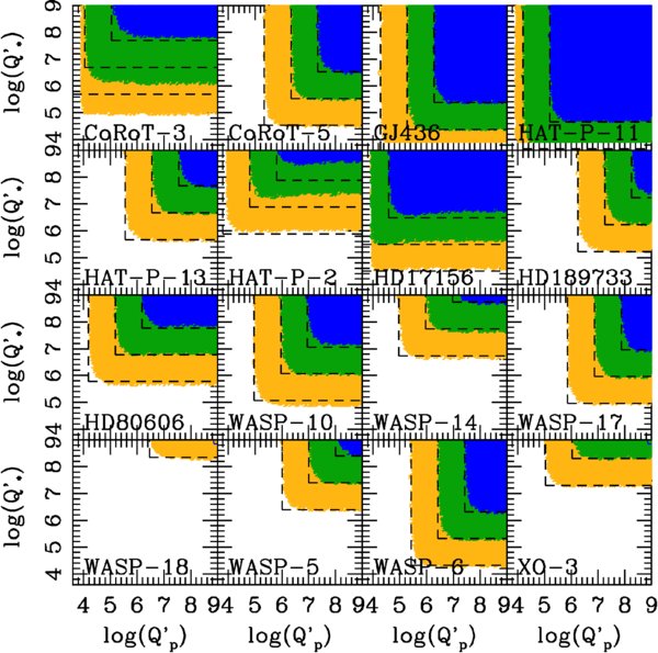
Figure 9. Same as Figure 7, but with the effects of magnetic braking included. There is very little difference for the future tidal evolutions with and without magnetic braking. The vertical and horizontal dashed lines are the same as in Figure 7.
Download figure:
Standard image High-resolution imageOne of them relates to the orbital distribution of planetary systems. Wright et al. (2009) compared the properties of multiple-planet systems with single-planet systems (i.e., with no obvious additional giant planet) and showed that their semimajor axis distributions are different. While single-planet systems have a double-peaked distribution, which is characterized by a pileup of giant planets between 0.03 and 0.07 AU (the so-called three-day pileup) as well as a jump in the number of planets beyond 1 AU, multiple-planet systems have a much more uniform distribution. They also pointed out that the occurrence of close-in (a < 0.07 AU) planets is lower for multiple-planet systems and that planets beyond 0.1 AU in multiple-planet systems exhibit somewhat smaller eccentricities compared to the corresponding single ones. If confirmed by future observations, this trend would favor planet–planet interaction scenarios over a migration one, because there is no obvious reason why the orbital distributions of single- and multiple-planet systems should be different for planet migration. On the other hand, gravitational interactions combined with tidal circularization may be able to explain such a difference, because strong gravitational interactions tend to disrupt the system, and thus currently observed multiple-planet systems are unlikely to have been strongly perturbed by stellar/planetary companions, and/or to have undergone catastrophic scattering events.
Another indication comes from the similarity between the stellar obliquity distribution derived from the observed systems and the distribution predicted by the Kozai migration scenario (Fabrycky & Tremaine 2007; Wu et al. 2007). Triaud et al. (2010) observed the RM effect for six transiting hot Jupiters and found that four of their targets appear to be in retrograde orbits with a projected stellar obliquity >90°. Combining the previous 20 systems with such measurements, they pointed out that 8 out of 26 systems are clearly misaligned and that 5 out of 8 misaligned systems exhibit retrograde orbits. They also derived the stellar obliquity distribution by assuming an isotropic distribution of the stellar spin with respect to the line of sight and found that the distribution closely matches that expected from the Kozai migration scenario (Fabrycky & Tremaine 2007; Wu et al. 2007). Fabrycky & Tremaine (2007) and Wu et al. (2007) independently studied the possibility of forming a close-in planet by considering the combined effects of secular perturbations due to a highly inclined distant companion star (i.e., Kozai-type perturbations) and tidal interactions with the central star. In this scenario, a Jupiter-mass planet which was initially on a nearly circular orbit at ∼5 AU can become a hot Jupiter. The mechanism involves a companion star on a highly inclined orbit (≃90°), which perturbs the planetary orbit and increases its eccentricity. Once the pericenter distance of the planet becomes small enough for tidal interactions with the central star to be important, energy dissipation leads to the circularization of the planetary orbit and eventually to the formation of a hot Jupiter with a small, or nearly zero, eccentricity. They found that hot Jupiters formed this way tend to be in misaligned orbits and frequently in retrograde orbits. Planet–planet interactions around a single star (without a binary companion) could also form hot Jupiters via Kozai migration (Nagasawa et al. 2008).
Yet another clue regarding the origin of close-in planets is related to the above scenario and comes from the inner edge of the orbital distribution for hot Jupiters. Ford & Rasio (2006) proposed that the observed inner cutoff for hot Jupiters is defined not by an orbital period, but by a tidal limit, and studied such a cutoff of the distribution of close-in giant planets in the mass–period diagram by performing a Bayesian analysis. Assuming that the cutoff slope in such a diagram follows the Roche limit, they found that the observations suggest an inner cutoff close to twice the Roche limit. This can be explained naturally if the planetary orbits were initially highly eccentric and later circularized via tidal dissipation while conserving orbital angular momentum. They suggested that this result is inconsistent with the migration scenario, because migration would lead to an inner edge right at the Roche limit (a factor of 2 closer to the star than what is observed).
In Figure 10, we extend the work of Ford & Rasio (2006) by including all more recently discovered planets and plot planetary and stellar mass ratio against the semimajor axis in terms of the Roche-limit separation (Paczyński 1971):
Here, we assume that the Roche radius of the planet, which is defined so that its spherical volume is equal to the volume within the Roche lobe, is equal to the planetary radius. Thus, the Roche-limit separation used here is the lower limit. For non-transiting planets without a measured planetary radius (orange circles), we assume a Jupiter radius for planets with mass larger than 0.01 MJ, and a Neptune radius for less massive planets. It is obvious that most planets still exist beyond twice the Roche limit (the vertical dashed line). However, there are now five planets which lie within this limit (OGLE-TR-56, CoRoT-1, WASP-4, WASP-19, and WASP-12) with a/aR ∼ 1.70, 1.67, 1.66, 1.30, and 1.24, respectively. We need to assess whether these planets will change the claim by Ford & Rasio (2006) and support the migration scenario over the scattering/Kozai-cycle scenario. Note that the two recently discovered "extreme" close-in planets, with orbital periods less than 1 day, CoRoT-7 b and WASP-18 b, have a/aR ∼ 2.76 and 3.52, respectively.
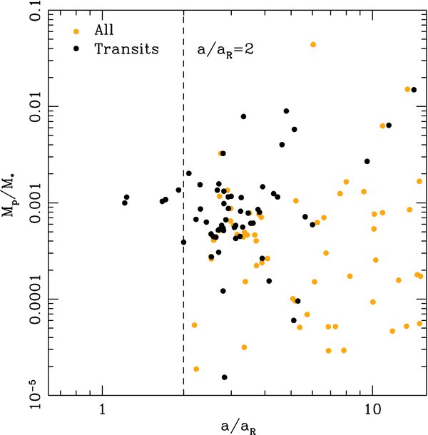
Figure 10. Planetary to stellar mass ratio as a function of semimajor axis normalized to the Roche-limit distance. For non-transiting planets (orange circles) without planetary radius information, we assume a Jupiter radius for planets with mass larger than 0.1 MJ, and a Neptune radius for planets with smaller mass. Most close-in planets lie beyond two times their Roche limit. One planet, WASP-12b, has a non-zero eccentricity and a very small semimajor axis (a ≃ 1.3aR).
Download figure:
Standard image High-resolution imageThe existence of at least some of these planets inside 2aR may still be explained as a result of the tidal circularization of an eccentric orbit. One of the possibilities is that the orbits of these planets were originally circularized beyond twice the Roche limit, but the planets have migrated inward after circularization due to the tidal dissipation in the star. All of the planets within 2aR can be potentially explained this way. Another possibility is that their orbits used to have a pericenter distance close to the Roche limit, but the initial eccentricity was smaller, e ≃ 0.7. In such a case, the expected period of the circularized orbit would be comparable to the current orbital period for OGLE-TR-56, CoRoT-1, and WASP-4, since they all have a/aR ∼ 1.7. However, systems with smaller ratios of the semimajor axis to Roche-limit separation (WASP-12 and WASP-19) are unlikely to be explained this way. This is because their current semimajor axes (a/aR ≃ 1.24 and 1.30) would demand small initial eccentricities (ei ∼ 0.24 and 0.30), and thus small initial semimajor axes (a0 ≃ 0.024 AU and 0.018 AU, respectively). This means that they have to be either born at such close-in locations, or scattered into such an orbit, which would be very difficult. Yet another possibility is that these planets used to have a smaller Roche-limit separation, due to a larger mass or a smaller radius. The orbits of these planets might have been circularized as the planet lost mass (e.g., Lammer et al. 2003; Lecavelier Des Etangs 2007), or the planetary radius expanded due to tidal heating (e.g., Bodenheimer et al. 2001; Gu et al. 2003). For OGLE-TR-56, CoRoT-1, WASP-4, WASP-19, and WASP-12 to be circularized at twice the Roche limit, either the past planetary masses must have been 2.13, 1.78, 1.53, 4.19, and 5.98 MJ, respectively, or the past planetary radii must have been 1.18, 1.24, 1.21, 0.829, and 1.11 RJ, respectively. Since the mass-loss rate can only be at most ∼10%, even for a low-density planet like WASP-12 (Lammer et al. 2009), it is unlikely that a larger mass in the past could be the correct explanation. On the other hand, tidal inflation of the planetary radius is a transient phenomenon (e.g., Ibgui & Burrows 2009). To explain the current orbital radius by invoking a smaller planetary radius in the past, we have to catch the planet just as its radius is inflating. Such a scenario may be possible, but appears unlikely. Interestingly, CoRoT-1 is observed to be strongly misaligned with λ = −77 ± 11 deg (Pont et al. 2010), which suggests a violent origin, while WASP-4 has a stellar obliquity of 4+34−43 deg (Triaud et al. 2010), which is consistent with alignment. We urge observers to determine the projected stellar obliquity for OGLE-TR-56, WASP-19, and WASP-12. Alignment does not necessarily support the planet migration scenario over the violent origin, but misalignment would clearly imply a significant past dynamical interaction involving scattering or Kozai cycles.
5.2. Past Evolution of Transiting Planets
As we pointed out in the previous section, planet–planet (or planet–companion star) interactions may well be responsible for the majority of close-in planets. Now we further explore this possibility by performing integrations of the tidal evolution equations backward in time. Particular focus is on the differences in evolution of Darwin-unstable planets depending on two evolution paths.
Jackson et al. (2008) first performed such a study and estimated the "initial" eccentricity distribution of close-in planets. They found that this distribution agrees well with the observed eccentricity distribution of exoplanets on wider orbits, and they proposed that most currently observed close-in planets had considerably wider and more eccentric orbits in the past. However, their study had many uncertainties. First, the possible effects of other planets and binary companions were neglected. As we pointed out in Section 2, these effects are most likely unimportant at present, but they could well have been playing a crucial role in the past, especially if another object was responsible for Kozai-type perturbations, or gravitational scattering. Second, the evolution of stars and planets is neglected. For example, both planetary and stellar radii may have been significantly different in the past. Moreover, many stars could have lost a large amount of their spin angular momentum via magnetic braking. Finally, such backward dynamical integrations of evolution equations with energy dissipation are known to be diverging, and thus small changes in initial conditions can lead to much larger changes in the calculated "initial" values.
With these caveats in mind, we now re-examine the possible past histories of transiting planets. Since Equations (7)–(11) are time-invariant, we can study the past evolution by integrating the differential equations "backward in time" (i.e., by taking the negative of these differential equations and integrating them from t = 0 to τage). For simplicity, we assume that the planetary spin is pseudosynchronized with the orbit at all times (i.e., dωp/dt = 0). First, we show typical results for WASP-18 in Figure 11. Here, the initial tidal quality factors are Q'*,0 = Q'p,0 = 106 with the scaling of Q' = Q'0n0/n, and the magnetic braking effect is neglected. As in Figure 6, solid curves show the results of backward evolution with the fiducial orbital parameters, while four dotted curves correspond to different combinations of maximum and minimum semimajor axis and eccentricity within uncertainties. The vertical dashed and dotted lines correspond to the estimated stellar age with uncertainties. As expected, both semimajor axis and eccentricity values differ significantly within uncertainties at the zero age (the vertical dashed line), or at any specific time within the age uncertainties (between the vertical dotted lines). However, we find that the fiducial case still provides a representative evolutionary path within the stellar age uncertainties. Figure 12 presents similar backward evolutions for all the systems shown in Figure 6. It is clear that, except for the Darwin-stable CoRoT-3, WASP-18 has the largest spread in orbital parameters within uncertainties. The backward evolution of the other systems is largely independent of the exact values of the orbital parameters.

Figure 11. Backward evolution of the semimajor axis a (black curves) and eccentricity e (orange curves) for WASP-18 with Q'*,0 = Q'p,0 = 106. The solid curves are the nominal values, and the dotted curves show four independent runs with different combinations of a and e within uncertainties. The vertical lines show the estimated stellar age with uncertainties.
Download figure:
Standard image High-resolution image
Figure 12. Same as the previous figure for other transiting systems. The evolution of the semimajor axis and eccentricity is shown with Q'*,0 = Q'p,0 = 106.
Download figure:
Standard image High-resolution imageNow we repeat backward integrations of the tidal equations by adopting various combinations of initial stellar and planetary tidal quality factors ranging over 104 ⩽ Q'0 ⩽ 109. This allows us to study the "initial" orbital properties at the zero stellar age (τage = 0) within the estimated age uncertainties. As in Section 4.3, we also assumed that each system initially has the currently observed orbital and rotational parameters.
We select systems that have solutions such that e < 1 somewhere in the interval τage,min ⩽ t ⩽ τage,max and plot the corresponding Q'*,0 and Q'p,0 values in Figure 13. Again, the tidal quality factors change as Q' = Q'0n0/n, and magnetic braking is neglected. The blue, green, orange, and red regions represent the maximum reachable "zero-age" semimajor axis for each system being 0.1, 1, 10 AU, and ⩾10 AU, respectively. The vertical and horizontal dashed lines are the same as in Figure 7 and indicate the minimum Q'p,0 and Q'*,0 required to have circularization and orbital decay times (i.e., the future survival time) of 0.1, 1, and 10 Gyr. As expected, when the tidal dissipation is inefficient in both the planet and the star (top right corner area of the figure), the planets are generally expected to have stayed where they are now for a long period of time. The lack of a significant change in its orbit, especially eccentricity, may be consistent with the initial orbital properties expected from the planet migration scenario. For the future survival time much longer than 10 Gyr, only such a solution with little migration is allowed in the parameter space. On the other hand, when tidal dissipation is highly efficient (bottom left corner), a planet could have started on a wide, eccentric orbit, which was then circularized over the lifetime of the system. The property of this area is in good agreement with the expectation from Kozai cycles and/or planet–planet interactions followed by tidal dissipation. The comparison of these regions with the dashed lines implies that most planetary systems have a large region of parameter space allowed for (Q'*,0, Q'p,0) which is consistent with having started on a wide, eccentric orbit, and with comfortable future survival times ∼1–10 Gyr. Thus, our results agree with the suggestion first made by Jackson et al. (2008) and show that there is a broad parameter space which supports the tidal circularization scenario as the dominant origin of close-in planets.
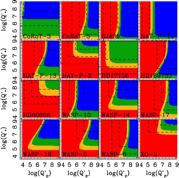
Figure 13. Combinations of stellar and planetary tidal quality factors that allow a planet to survive (i.e., e < 1) for the stellar age with uncertainties in backward integration of the tidal equations. Magnetic braking is not included, and tidal quality factors change as Q' = Q'0n0/n. The blue, green, orange, and red areas correspond to a maximum zero-age semimajor axis of 0.1, 1, 10, and ⩾10 AU, respectively. Also plotted are the same vertical and horizontal dashed lines shown in Figure 7.
Download figure:
Standard image High-resolution imageWhen we demand that the future survival time must be comparable to or slightly longer than the estimated stellar age, Figure 13 implies an interesting trend. In the stellar-dissipation-dominated region, planets tend to have an initial orbit which is similar to the current one, while in the planetary-dissipation-dominated region, planets tend to have an initially highly eccentric and wide orbit. This is clear by comparing these two regions (below and above the diagonal line that can be drawn by connecting the vertices of the vertical and horizontal dashed lines) at around their survival times. Most systems in the figure except WASP-10, WASP-14, WASP-18, and WASP-6 have the estimated age of ∼1–10 Gyr, while WASP-10, WASP-14, and WASP-18 have ∼0.1–1 Gyr, and WASP-6 has >10 Gyr. Investigating the corresponding regions, we find that the maximum zero-age semimajor axis can be very large (up to >10 AU) in the planetary-dissipation-dominated region. On the other hand, such a solution is less likely in the stellar-dissipation-dominated region, and the area with a little change in orbital radii tends to occupy the largest region of parameter space.
Figure 14 presents similar results with magnetic braking effects included. As we can see, some systems are much less affected by magnetic braking than others. Our results show that, when either the stellar spin is slow, or the mass ratio is very low, the evolution is less affected by magnetic braking. Clearly affected systems include CoRoT-3, HAT-P-2, HD 189733, WASP-10, WASP-14, WASP-18, WASP-5, and XO-3, for which the average stellar spin period is ≃8 days and the average mass ratio is ≃0.006, while the corresponding values are about 36 days and 0.001 for the others.
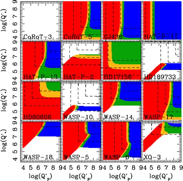
Figure 14. Same as Figure 13, but with the effects of magnetic braking included. Systems that are affected the most by magnetic braking have a rapidly rotating star, and/or a relatively high mass ratio. For CoRoT-3, we do not get any solutions.
Download figure:
Standard image High-resolution image5.3. Stellar Obliquity Evolution
Figures 15 and 16 show similar plots to Figures 13 and 14 for the stellar obliquity. The blue, green, orange, and red areas correspond to a maximum possible zero-age obliquity of 5°, 20°, 40°, or ⩾40°. Again, also plotted are the same vertical and horizontal lines as in Figure 7.
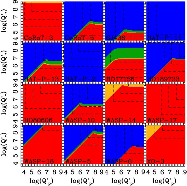
Figure 15. Combinations of stellar and planetary tidal quality factors that allow a planet to survive (i.e., e < 1) for the stellar age with uncertainties in backward integrations of the tidal equations. Magnetic braking is not included, and tidal quality factors are scaled as Q' = Q'0n0/n. The blue, green, orange, and red areas correspond to a maximum zero-age stellar obliquity of 5, 20, 40, and ⩾40 deg, respectively. Also, plotted for reference are the same vertical and horizontal dashed lines shown in Figure 7.
Download figure:
Standard image High-resolution image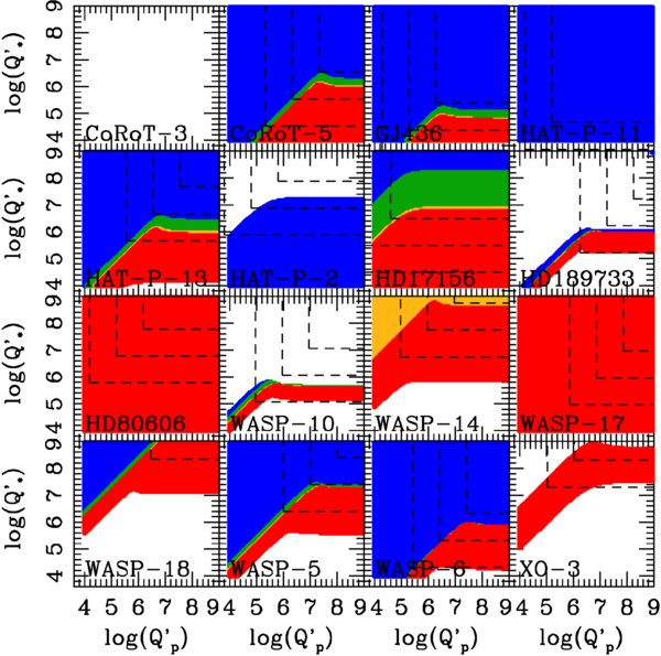
Figure 16. Same as Figure 15, but with magnetic braking included. Systems which are affected the most have a rapidly rotating star, and/or a relatively high mass ratio. For CoRoT-3, we do not get any solutions.
Download figure:
Standard image High-resolution imageIn Figures 15 and 16, CoRoT-3, HAT-P-2, HD 17156, HD 80606, WASP-14, WASP-17, WASP-18, WASP-5, WASP-6, and XO-3 have RM measurements, and thus known projected stellar obliquities. Among them, CoRoT-3, HD 80606, WASP-14, WASP-17, and XO-3 have a significant misalignment (>20°). Naturally, the maximum possible misalignment at zero age can be very large (⩾40°) for these systems with almost any values of (Q'*, Q'p). On the other hand, for systems with small measured projected obliquities (HAT-P-2, HD 17156, WASP-18, WASP-5, and WASP-6), or systems with no RM measurements (CoRoT-5, GJ 436, HAT-P-11, HAT-P-13, HD 189733, and WASP-10), we find either a little or large change in obliquity over the stellar age.
Consider a few specific cases. For HAT-P-2 and HAT-P-11, there are no solutions for obliquity larger than 5°. This indicates that, for HAT-P-2, the "zero-age" obliquity was likely similar to the current nominal value λ = 12. However, since HAT-P-2's measured obliquity has a very large uncertainty (λ = 12 ± 134), it is possible that the actual present value is much larger. Note that even if the stellar obliquity turns out to be small, HAT-P-2 is still likely to have the scattering/Kozai-cycle origin. This is partly because of its high eccentricity (e ∼ 0.52) and partly because of a large range of tidal quality factors that allow a much wider orbit in the past (see Figures 13 and 14). For HAT-P-11, there are no RM measurements thus far, but the system shows a similar result to HAT-P-2 with *,0 = 2°. If the current obliquity turns out to be ≲2°, our plot indicates that HAT-P-11 would not have had a large obliquity in the past. This in turn indicates that, if HAT-P-11 initially had a large stellar obliquity, we should be able to see a clearly misaligned orbit through future observations, independent of the actual tidal quality factors for the system. The orbital eccentricity of the planet is e = 0.198 ± 0.046, which could have been produced either via planet–disk or planet–companion interactions. Interestingly, Figures 13 and 14 show that the orbital radius of HAT-P-11 b is unlikely to have been changed significantly via tidal evolution, unless the tidal dissipation inside the planet is rather efficient (Q'p < 106). If the tidal dissipation is inefficient, our result suggests that HAT-P-11 b is likely to have migrated in a disk. We have to wait for future observations to estimate whether the planet is likely formed via disk migration or tidal circularization of a highly eccentric orbit.6
For all the other systems, the zero-age obliquity can be as high as ⩾40° if stellar tidal quality factors are relatively small. More specifically, such solutions are allowed in the stellar-dissipation-dominated region with τe ≃ τa. The stellar obliquity generally damps on a similar timescale to the orbital decay (see, e.g., LWC09; Barker & Ogilvie 2009, as well as Section 4.1). However, this plot demonstrates that the stellar obliquity could be damped from high (≳40°) to low (∼2°) values within the current stellar age.
Note that these small stellar tidal quality factors, which allow the fast damping of stellar obliquities, also lead to relatively short survival times for planets. By comparing these zero-age high-obliquity regions with the horizontal dashed lines, we find that these tidal quality factors lead to survival times comparable at most to the current stellar age. In other words, a relatively small region of parameter space is allowed for these high zero-age obliquities. For example, when we demand that the expected survival time in forward tidal evolution must be comparable to or larger than the stellar age, we find that the stellar tidal quality factor for CoRoT-5 must be Q'* ≳ 106. This includes a small region of the red, large "zero-age" stellar obliquity area in Figure 15. However, if Q'* ≳ 107, such an area disappears. In the latter case, if the observations find a small stellar obliquity for CoRoT-5, it is unlikely that the stellar obliquity was much larger in the past. In some cases, such a region with a high zero-age obliquity and a comfortable future survival time may not even exist. For HAT-P-13, a similar comparison shows that the stellar tidal quality factor must be Q'* ≳ 107 for the survival time to be comparable to or larger than the stellar age. This corresponds to the blue, small "zero-age" stellar obliquity area in Figure 15, and thus we expect that the stellar obliquity of HAT-P-13 could not have been changed much due to tidal evolution (i.e., similar to HAT-P-2 or HAT-P-11). Interestingly, HAT-P-13 is the only system in our sample that has an additional planetary companion. Thus, the system may be an example of a close-in planet formed via migration scenario. If this is the case, we predict the future observations will find a small stellar obliquity for HAT-P-13.7
In short, by comparing Figure 13 with Figure 15, we find that the evolution history is largely divided into two cases, depending on the relative efficiency of energy dissipation inside the star and the planet. In the planetary-dissipation-dominated region, the planets could have had a wide, eccentric orbit in the past, and the stellar obliquity damps on a similar timescale to the orbital decay. The initial conditions implied in this region are consistent with those expected from the scattering/Kozai-cycle origin of the close-in planets. On the other hand, in the stellar-dissipation-dominated region, the system could have had a large stellar obliquity in the past, although the initial orbital radius and eccentricity are likely similar to the current values, as planet migration scenario would suggest. Further inspection of these figures shows that a unique evolution is possible in the transition region between these two, where the dissipation effects due to the planet and a star are comparable. There, the system could have had a wide, eccentric orbit, as well as a large stellar obliquity in the past. Our results also imply that if the currently observed stellar obliquity distribution is due to Kozai migration, as suggested by Triaud et al. (2010), then most exoplanetary systems have planetary-dissipation-dominated tidal interactions (i.e., τe < τa). If τe ≃ τa for most planetary systems, the current obliquity distribution should be very different from the initial one, and any memory of the dynamical history prior to the tidal dissipation should be erased.
Recently, Winn et al. (2010a) suggested that the stellar obliquity is preferentially large for hot stars with effective temperatures Teff>6250 K and proposed that such a trend can be explained because photospheres of cool stars can realign with the orbits due to tidal dissipation in the convective zones, without affecting the orbital decay. Our results suggest that yet another possibility might be that the evolution of the systems with hot and cool stars corresponds to slow and fast obliquity damping regions, respectively. If that is the case, the stellar obliquity may stay nearly constant for the planetary systems with a hot star, because tidal dissipation is dominated by the planet (i.e., τe < τa), while the obliquity may be damped to a small value for the systems with a cool star, because tidal dissipation is either dominated by the star (i.e., τe ≃ τa), or the star and the planet have comparable dissipation. In our samples of eccentric systems, CoRoT-5, GJ 436, HAT-P-11, HAT-P-13, HD 17156, HD 189733, HD 80606, WASP-10, WASP-5, and WASP-6 have the effective temperatures less than 6250 K. For the range of tidal quality factors we use, we do not see any trend that these cool systems prefer τe ≃ τa. One possibly interesting example is HD 17156, for which a large region of parameter space is allowed for the stellar-dissipation-dominated case (τe ≃ τa).
6. DIFFERENT SCALINGS FOR TIDAL QUALITY FACTORS
So far, we have focused on a scaling of Q ∝ 1/n. However, this scaling is not appropriate unless a close-in planet system reaches a true dual synchronization of n = ω* = ωp. This cannot be reached unless both eccentricity and obliquities are zero, or some extra torques are acting on the system. For a planetary spin, although the true synchronization with the orbit normal does not occur until the final spiral-in of the planet, pseudosynchronization is reached quickly (see, e.g., Sections 4.1 and 4.2). On the other hand, stellar spin changes on a similar timescale to the orbital decay, and thus it is reasonable, for most systems, to assume that the stellar spin is far from synchronization. As we have seen in Section 3.1, the semidiurnal tide with the forcing frequency of |2ω − 2n| dominates the energy dissipation before the spin–orbit synchronization, while the annual tide with |2ω − n| takes over once the synchronization approaches. Therefore, in this section, we scale the planetary and stellar tidal quality factors as Qp ∝ 1/|2ωp − n| and Q* ∝ 1/|2ω* − 2n|, respectively, and investigate the differences in future and past evolution from the results of the scaling Q ∝ 1/n.
In Figure 17, we repeat the similar tidal evolution forward in time as Figure 7 with the initial tidal quality factors ranging over the interval 104 ⩽ Q'0 ⩽ 109. The figure has a similar general trend to Figure 7, but a larger region of parameter space is allowed. The vertical and horizontal lines are obtained by rescaling Equations (17) and (18) by n0/|2ωp,0 − n0| and n0/|2ω*,0 − n0|, respectively. The agreement with the integration of the complete tidal equations is pretty good.

Figure 17. Same as Figure 7, but with different scaling for tidal quality factors. See text for details.
Download figure:
Standard image High-resolution imageSimilarly, Figures 18 and 19 show the corresponding results to Figures 13 and 15, respectively, with the modified Q scalings. Both of these figures have a good agreement with the Q ∝ 1/n case.
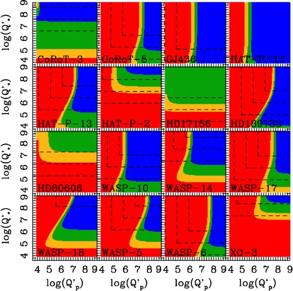
Figure 18. Same as Figure 13, but with different scaling for tidal quality factors. See text for details.
Download figure:
Standard image High-resolution image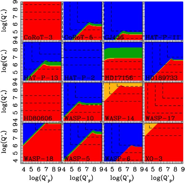
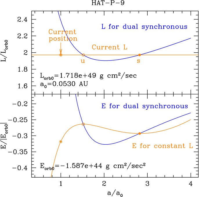
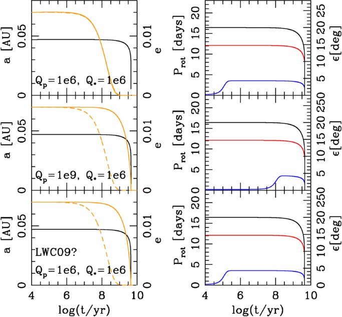
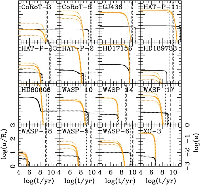
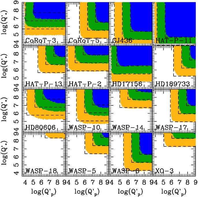
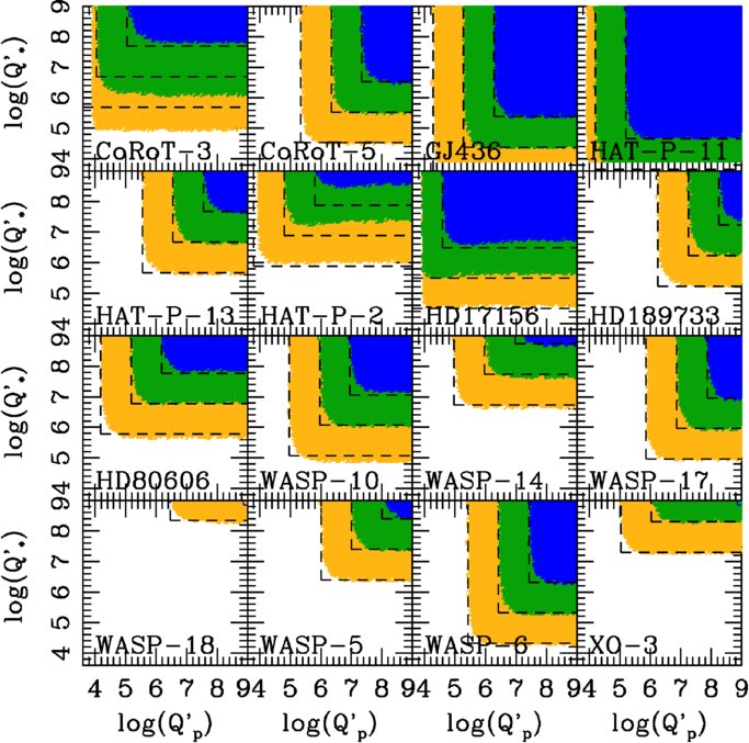
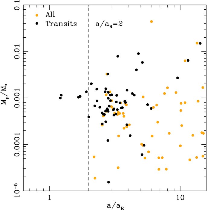
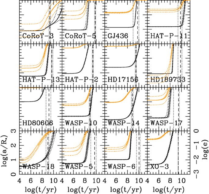
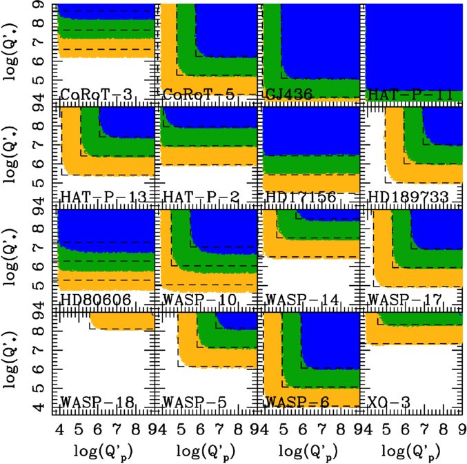
Figure 19. Same as Figure 15, but with different scaling for tidal quality factors. See text for details.
Download figure:
Standard image High-resolution image
7. DISCUSSION AND CONCLUSIONS
Close-in planets may be formed via planet migration in a disk, or via tidal circularization of a highly eccentric orbit following planet–planet scattering or other gravitational interactions with a companion. There is strong observational support for the tidal circularization scenario. First, the current observations exhibit different orbital distributions for apparently single- and multiple-planet systems (Wright et al. 2009). The so-called three-day pileup and a jump in planetary abundance beyond 1 AU are not seen among multi-planet systems. It is difficult to explain such a difference as a result of planet migration, since migration in the disk without strong planet–planet interactions is expected to lead to similar orbital distributions for both single and multiple-planet systems. On the other hand, strong gravitational interactions between planets and/or with stellar companions can disrupt the multiple-planet systems by ejecting planets or scattering them far away from one another. Thus, from such a scenario, it is expected that systems which have gone through violent dynamical interactions have only one planet close to the central star, while systems which did not experience such an event retain multiple planets close-by. Second, the observed distribution of stellar obliquities matches very well with the expectation from Kozai migration (Triaud et al. 2010). Third, the observed inner edge of the orbital distribution is not at the Roche limit aR, which would be expected from planet migration, but rather at 2aR, which is naturally explained by the circularization of a highly eccentric orbit while conserving orbital angular momentum (Ford & Rasio 2006).
In this paper, we have further explored the possibility of forming close-in planets via tidal circularization of an eccentric orbit by studying the past and future evolutions of eccentric transiting planets. We considered a broad range of tidal quality factors, ∼104–109, consistent with our limited theoretical understanding of tidal dissipation in both stars and planets. We have used a tidal model where Q' ∝ 1/(σΔt) as the simplest representation because of the unknown character of tidal dissipation in stars and gaseous planets. Our choice is consistent with the constant time lag model (Hut 1981) that is derived as a quadrupolar approximation of the tidal potential. Although different tidal models can change the timescales of the various processes, the qualitative properties of the evolution should be the same as other models. Another caveat here is that, for these close-in planets, the ratio R*/a is relatively large and often ∼0.1 (e.g., see Figure 6). Thus, the higher order terms in the tidal potential can be important, as they are for Mars' satellites Phobos and Deimos (e.g., Bills et al. 2005).
In Section 2, we investigated the effects of (known or unknown) planetary/stellar companions on the evolution of observed close-in planets. Comparing secular timescales with GR precession timescales, we showed that the current and future evolutions of most close-in planets are unlikely to be strongly affected by such companions. In Section 4.1, we re-examined the tidal stability of transiting systems and confirmed that the majority of close-in planets are Darwin unstable. The exceptions include CoRoT-3, CoRoT-6, HD 80606, and WASP-7, which are Darwin stable within the current observational uncertainties. We also found that borderline cases such as HAT-P-2 and WASP-10 are most likely Darwin unstable, but could be Darwin stable within the uncertainties.
For clearly Darwin-unstable systems (with Ltot ≪ Lcrit), there are two possible evolutionary paths. When the tidal dissipation in the star dominates the evolution, all parameters but the planetary spin evolve on a similar timescale ( ). On the other hand, when tidal dissipation in the planet is non-negligible, the orbit tends to get circularized before the planet spirals all the way to the Roche limit (
 ). Although it is nontrivial to determine which evolutionary path each system will take without knowing the efficiencies of tidal dissipation in the star and in the planet, there are some indications that the dissipation in the planet dominates (τe < τa) for most systems. First, there is clear evidence of eccentricity damping within ∼0.1 AU. Most observed close-in planets are on nearly circular orbits, which are well described by the traditional exponential eccentricity damping approximation. Second, our results in Section 5.2 suggest that we need to assume τe < τa for most systems in order to explain the current obliquity distribution through Kozai migration. With stellar-dissipation-dominated cases (τe ∼ τa), we expect that the distribution of current stellar obliquity would be significantly different from the one expected from Kozai migration.
In Section 4.3, we showed that the lifetime of the planetary systems is largely determined by the tidal dissipation in the star, while the circularization time is largely determined by the dissipation in the planet. Also, we confirmed the results of Barker & Ogilvie (2009) and showed that magnetic braking does not have a large effect on future evolution, except in systems with a rapidly rotating star. The minimum stellar tidal quality factor that allows a planet to survive for a certain age is similar for the cases with and without magnetic braking (see Figures 7 and 9).
In Section 5, we found that, generally speaking, the evolution history in the stellar-dissipation-dominated tidal evolution is consistent with that expected from the planet migration origin of close-in planets, with a little change in the semimajor axis and eccentricity over the stellar age. On the other hand, the evolution history in the planetary-dissipation-dominated evolution is consistent with that expected from scattering/Kozai-cycle origin, with initial orbits being wide and eccentric. The latter case agrees with the results in Jackson et al. (2008). We also showed that, when the effects of tidal dissipation in the star are comparable to, or larger than those in the planet, the stellar obliquities could be damped from high ≳40° to low ∼2° values within the currently observed stellar ages (see Figures 15 and 16).
Overall, our results for the tidal evolution of eccentric transiting planets are consistent with the formation path that involves the circularization of an initially eccentric orbit. The distribution of system parameters seems to imply that this mechanism dominates for close, single-planet systems, but multi-planet systems are more consistent with a disk-migration origin for their close-in members.
This work was supported by an Astronomy Center for Theory and Computation Prize Fellowship (to S.M.) at the University of Maryland and by NSF Grant AST-0507727 (to F.A.R.) at Northwestern University. Partial support was also provided by the Center for Interdisciplinary Exploration and Research in Astrophysics (CIERA) at Northwestern University. S.J.P. is supported in part by NASA under grant NNG06GF42G in the Origins of Solar Systems Program. S.M. also thanks the support from the Kavli Institute for Theoretical Physics at UC Santa Barbara while part of this work was done. We thank Benjamin Levrard, Gilles Chabrier, Brian Jackson, Amaury Triaud, Dong Lai, Yoram Lithwick, and Smadar Naoz for useful discussions, and an anonymous referee for valuable comments on the manuscript. S.M. thanks Genya Takeda for making the time comparison code used in Figures 1 and 2 available.
Footnotes
- 5
Note that the choice of the factor is rather arbitrary. The exact number can be anything as long as the planetary contribution becomes negligible compared to the stellar contribution.
- 6
As we were completing the final revision of this paper, two groups released results showing that HAT-P-11 is a highly inclined system. The sky-projected stellar obliquity is λ = 103+26−10 deg by Winn et al. (2010c) and 103+23−19 deg by Hirano et al. (2010). Thus, the system is likely to have originated from planet–planet scattering and/or Kozai cycles, rather than migration in a disk.
- 7
Indeed, a recent observation found a well-aligned orbit for HAT-P-13b with λ = −1.9 ± 8.6 deg (Winn et al. 2010b).