


ABSTRACT
We present a three-dimensional density model of coronal prominence cavities, and a morphological fit that has been tightly constrained by a uniquely well-observed cavity. Observations were obtained as part of an International Heliophysical Year campaign by instruments from a variety of space- and ground-based observatories, spanning wavelengths from radio to soft X-ray to integrated white light. From these data it is clear that the prominence cavity is the limb manifestation of a longitudinally extended polar-crown filament channel, and that the cavity is a region of low density relative to the surrounding corona. As a first step toward quantifying density and temperature from campaign spectroscopic data, we establish the three-dimensional morphology of the cavity. This is critical for taking line-of-sight projection effects into account, since cavities are not localized in the plane of the sky and the corona is optically thin. We have augmented a global coronal streamer model to include a tunnel-like cavity with elliptical cross-section and a Gaussian variation of height along the tunnel length. We have developed a semi-automated routine that fits ellipses to cross-sections of the cavity as it rotates past the solar limb, and have applied it to Extreme Ultraviolet Imager observations from the two Solar Terrestrial Relations Observatory spacecraft. This defines the morphological parameters of our model, from which we reproduce forward-modeled cavity observables. We find that cavity morphology and orientation, in combination with the viewpoints of the observing spacecraft, explain the observed variation in cavity visibility for the east versus west limbs.
Export citation and abstract BibTeX RIS
1. INTRODUCTION
Coronal mass ejections (CMEs) are spectacular solar eruptions and the primary drivers of "space weather" at the Earth (Pick et al. 2006; Hudson et al. 2006). CMEs are most commonly observed in white light, and many possess the classic "three-part" morphology of a bright expanding loop, followed by a relatively dark cavity, and lastly a bright core associated with an erupting prominence. Such three-part CMEs have been observed to erupt from previously quiescent cavities with embedded prominences (Sterling & Moore 2004; Gibson et al. 2006). Indeed, prominences and cavities are ubiquitous features of the non-erupting corona: several may be visible on any given day. In the polar crown they can be long-lived (on the order of months), either reforming after or only partly erupting in CMEs (Gibson & Fan 2006; Su et al. 2006; Liu et al. 2007; Tripathi et al. 2007, 2009). Prominences and their cavities thus provide clues to magnetohydrodynamic (MHD) equilibrium states of the solar corona and to the processes which can destabilize these equilibria and drive certain CMEs.
The thermodynamic properties of cavities provide information about their magnetic structure and MHD equilibrium: for example, Zhang & Low (2004) model a low-density cavity which is hotter than its surroundings, and van Ballegooijen & Cranmer (2008) demonstrate how different heating mechanisms lead to different distributions of density and temperature in the cavity. Flows within and between prominences and cavities likewise have implication for their magnetic structure (van Ballegooijen & Cranmer 2010). It is therefore critical to obtain information about cavity plasma density, velocity, and temperature via multi-wavelength observations in order to test and constrain MHD models.
Cavity densities are most unambiguously determined from white-light observations, which are temperature-independent, and these indicate that cavity density has a lower limit of approximately half the density of a surrounding streamer at the same height (Fuller et al. 2008; Fuller & Gibson 2009). Radio observations have been consistent with this (Marqué 2004 and references therein).
Studies of velocities associated with the non-erupting cavity have more recently been undertaken: Schmit et al. (2009) observed large-scale flows on the order of 5–10 km s−1 in coronal cavities using extreme ultraviolet (EUV) and infrared spectroscopy. Spinning motions within cavities have also been observed, with a preferred direction of spin consistent with meridional flows (near solar minimum; Wang & Stenborg 2010).
Temperature determination of cavities is a more challenging problem. From white light, the only information that can be obtained is an inferred density scale height and associated "hydrostatic temperature" (Guhathakurta et al. 1992). A comparison of white-light scale heights in cavities versus their surrounding streamers indicates a higher hydrostatic temperature for most cavities (Fuller et al. 2008; Fuller & Gibson 2009). Since hydrostatic balance is along magnetic flux tubes, however, this implicitly assumes a uniform lower boundary density for all flux tubes that intersect the radial cuts along which scale heights are determined. This assumption may be particularly unsuitable for prominences and their cavities: indeed, an isothermal, MHD simulation of an emerging magnetic flux rope showed that density variations at the lower boundary led to differing cavity versus streamer density scale heights as observed in white light, with no need for enhancement of cavity temperature (Fuller et al. 2008).
Independent information about cavity temperature can be obtained from observations of emission due to coronal spectral lines. Guhathakurta et al. (1992) examined densities and temperatures in a coronal cavity using eclipse observations in white light and the coronal red (6374 Å Fe x) and green (5303 Å Fe xiv) lines. The white-light data indicated a clear density depletion, and, as in the Fuller et al. (2008) analysis, a hydrostatic temperature hotter than the streamer. On the other hand, their analysis of the line ratio of the red and green lines, a measurement which does not make hydrostatic assumptions, indicated cooler temperatures in the cavity. More recently, Habbal et al. (2010) used eclipse observations in white light and a range of iron lines to argue that low-emission regions around prominences were hot relative to the surrounding corona. However, the white-light observations associated with these structures indicated little or no density depletion. Thus, as the authors pointed out, they were not good examples of "cavities" in the sense of a lack of density, despite the fact that there was low emission at some wavelengths surrounding the prominence. Because the corona is optically thin, the orientation and three-dimensional morphology of the cavity may result in a large fraction of the line of sight being filled with non-cavity plasma, impacting both density depletion and temperature diagnostics. Thus, it is important to consider the three-dimensional morphology of any given cavity to understand the line-of-sight projection effects.
One approach for dealing with such projection effects is tomographic reconstruction, which requires no assumptions about boundary conditions or cavity morphology and explicitly accounts for line-of-sight effects. Vasquez et al. (2009, 2010) used STEREO EUVI images to tomographically reconstruct coronal cavities, and found differential emission measure (DEM) consistent with lower density and higher temperature in the cavity than in the surrounding corona. This is the strongest evidence for "hot" cavities to date (in cavities which are demonstrably low density), although it must be noted that these analyses have so far been limited to three Extreme Ultraviolet Imager (EUVI) bandpasses which cannot define a complicated DEM (Schmelz et al. 2007). It is possible that cavity temperature may vary internally, with only sub-regions being particularly hot—for example, near the cavity center where soft X-ray (SXR) emission has been observed surrounded by an otherwise low-emission cavity (Hudson et al. 1999; Hudson & Schwenn 2000). (The "hot shrouds" around prominences observed by Habbal et al. (2010) could also have their origin in such structures.) Observations with broad spectral range, plane-of-sky spatial resolution, and information about the cavity in three dimensions are required to conclusively establish cavity temperature relative to the surrounding corona.
In this paper, we present observations of a coronal cavity observed in 2007 August during a multi-instrument observing campaign organized under the auspices of the International Heliophysical Year (IHY). These observations represent the most comprehensive observations of a cavity yet taken, at wavelengths ranging from radio to SXR and with cavity-specific spectroscopic density and temperature diagnostics. Our ultimate goal is to use these diagnostics and observations of the full range of wavelengths to constrain a forward model of the three-dimensional density and temperature of the cavity. As a first step, in this paper we will determine the cavity's three-dimensional morphology (eight free parameters, described below), using observations taken from a range of wavelengths and viewing angles. In Section 2, we will describe the data taken during the IHY campaign, and demonstrate that our cavity is a region of low density and that it extends in longitude. In Section 3, we present our model and fit it to the data. In Section 4, we use the results of the forward model to examine how integration along the line of sight may produce differences in cavity visibility for different viewpoints. In Section 5, we present our conclusions.
2. IHY CAMPAIGN ON CORONAL PROMINENCE CAVITIES, 2007 AUGUST 8–18
As described above, quantitative studies of density and temperature to date have primarily been done using radio and white-light observations. Cavities have also been observed in the emission corona at EUV and SXR wavelengths (Hudson et al. 1999; Hudson & Schwenn 2000; Sterling & Moore 2004; Heinzel et al. 2008). To our knowledge, the IHY campaign was the first time a campaign was run with targetted observing plans customized for cavity density/temperature spectral diagnostics, with long integration times and a broad spectral range. It is essential to consider the three-dimensional morphology and orientation of cavities, to properly account for projection effects of non-cavity material into the line of sight (Wiik et al. 1994; Fuller et al. 2008). A critical campaign goal thus was to obtain multiple views and observations at a broad range of wavelengths, in order to constrain the three-dimensional morphology of the cavity and its surrounding streamer.
Campaign observations included white-light polarized brightness (pB) data from Mauna Loa Solar Observatory (MLSO) Mk4 K-coronameter (Elmore et al. 2003), SXR data from the Geostationary Operational Environmental Satellite (GOES) Solar X-Ray Imager (SXI; Hill et al. 2005), EUV image data from STEREO Sun Earth Connection Coronal and Heliospheric Investigation (SECCHI) EUVI A and B (Howard et al. 2008), Solar and Heliospheric Observatory (SOHO) Extreme ultraviolet Imaging Telescope (EIT; Delaboudiniere et al. 1995) and the Transition Region and Coronal Explorer (TRACE; Golub et al. 1999), UV and EUV spectroscopic data from SOHO Coronal Diagnostic Spectrometer (CDS; Harrison et al. 1996), and Hinode Extreme ultraviolet Imaging Spectrometer (EIS; Culhane et al. 2007), and radio observations from the Nançay Radioheliograph (Kerdraon & Delouis 1997). We have also made use of Hα synoptic charts to determine the location of filament channels and magnetic neutral lines on the disk (McIntosh 2003).
We observed portions of a well-established and longitudinally extended polar-crown filament channel (PCFC) over the period 2007 August 7–18. Targetted observations took place at the northeast limb (August 8–13), central meridian (August 14), and at the northwest limb (August 15–18). The portions of the PCFC we observed contained a prominence at least part of the time and were clearly associated with a cavity at the northeast limb (see Figure 1). For reasons we will discuss in Section 4, the cavity was not clearly visible when it rotated around to the northwest limb. Our analysis therefore focuses on fitting the model to observations of the cavity at the northeast limb.

Figure 1. 195 Å images of cavity from STEREO EUVI-A ((a)–(f)) 2007 August 7–12. Numbers below the time stamp indicate Carrington longitude at the east limb on that day (90° less than the central meridian Carrington longitude).
Download figure:
Standard image High-resolution image2.1. Cavity Variation with Wavelength
Figure 2 shows observations of the cavity on 2007 August 9 near 00:00:00 UT, when it was clearly visible at the NE limb. Although there is some variation of bright substructures within the cavity, the basic size and shape of the cavity do not vary much with wavelength. Observations shown are from similar times, but range in wavelength and hence plasma-temperature sensitivity. The EUV 171 Å observations have a peak temperature response at  , and the 284 Å observations have a peak temperature response at
  (Dere et al. 2000; Howard et al. 2008). GOES-SXI has a broad temperature response at SXR wavelengths, and is sensitive to plasmas of temperatures greater than ∼1 or 2 MK, with the sensitivity increasing somewhat with temperature up to ∼10 MK (Pizzo et al. 2005).
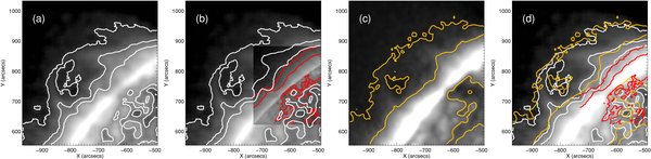
Figure 2. Cavity on 2007 August 9 at a range of wavelengths: (a) SOHO EIT 284 Å, 01:04:50 UT (gray scale and white contours); (b) TRACE 171 Å, 00:01:55 UT (inner image gray scale and red contours) embedded in EIT 284 Å (outer image gray scale and white contours); (c) GOES-SXI, 00:03:06 UT (gray scale and yellow contours); (d) EIT 284 Å (gray scale) with all three contours overplotted.
Download figure:
Standard image High-resolution imageFigure 3 shows TRACE 171 Å and GOES SXI data from approximately 24 hr later. We have bracketed the edge of the cavity at three radial heights, and show these edges overplotted on intensity versus colatitude profiles. As discussed in Gibson et al. (2006), the edges measured "by eye" in the images basically correspond to inflection points in the intensity plots. The SXI cavity appears somewhat more compact, with a more sharply defined poleward boundary, but its overall size and shape are similar to the cooler, 171 Å cavity. This indicates that the intensity gradient between the cavity and the surrounding corona is likely to be primarily a density, rather than a temperature effect. Near the embedded prominence, however, the EUV lines must be interpreted carefully. First of all, a lack of emission could be due to either a density depletion or to absorption by dense, relatively cool prominence material. Second, transition region and coronal emission may occur in the vicinity of a prominence; for example, Kucera & Landi (2006) reported emission in spectral lines produced at log T = 5.8 associated with an activated prominence (see also Labrosse et al. 2010). This temperature is near the peak response of the 171 Å bandpass, and so this may explain the central bump in intensity versus colatitude in Figures 3(a) and (c). Figure 4(a) also shows 284 Å emission colocated with the central prominence, and this may also in part be due to the presence of some transition-region lines in that bandpass (see Figure 12 in Dere et al. 2000 and Figure 7 in Howard et al. 2008). Alternatively, the 284 Å emission may be related to so-called chewy nougats, large regions of hot material (approaching ≈2 MK) interior to cavities observed in SXR (Hudson et al. 1999; Hudson & Schwenn 2000). Temperature variation may therefore play a significant role in creating substructures within the cavity. However, we note again that the outer boundary of the cavity has similar location and shape at all wavelengths (SXR, 171, 195, and 284 Å), indicating that, substructure aside, we are observing a true cavity (i.e., a density depletion).
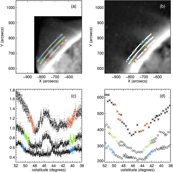
Figure 3. (a) TRACE 171 (August 9, 19:46:20 UT) and (b) SXI (August 10, 00:03:06 UT) observations of the cavity. (c) TRACE 171 intensity vs. colatitude (north pole is to the right) and (d) SXI intensity vs. colatitude corresponding to radial cuts shown in (a) and (b), respectively. Note that increasing radial heights in (a) and (b) correspond to decreasing intensities in (c) and (d). Colored regions indicate edge of cavity determined from images in (a) and (b), with corresponding colatitude ranges indicated in (c) and (d).
Download figure:
Standard image High-resolution image
Figure 4. Cavity and associated prominence observed by EIT on 2007 August 10: (a) 284 Å (01:06 UT) and (b) 304 Å (01:19 UT).
Download figure:
Standard image High-resolution image2.2. Density Depletion in Cavity
As noted above, radio and white-light observations have historically been used to demonstrate low density in cavities relative to surrounding material. The cavity we are observing is rather small compared to those that tend to be studied in white light, which are biased toward sizes easily seen above a coronagraph occulting disk (Gibson et al. 2006). Figure 5(a) illustrates this—the white-light streamer is a much bigger structure than the cavity, which is visible as a faint depletion near the coronagraph occulting disk (see also Figure 5(b)). The location of the cavity within the global white-light structure is indicated by an insert showing a density–sensitive line ratio (Fe xii 186/195 Å) obtained by Hinode EIS. This line ratio is related to line-of-sight-averaged density, and is indeed lower in the cavity than its surroundings (Figure 5(c)). Figure 5(b) shows the cavity in white light (polarized brightness), which is proportional to electron density integrated along the line of sight, and which also indicates depleted density in the cavity. For both of these measurements, some sort of assumption about variation of density along the line of sight is required to quantify plane-of-sky density. The three-dimensional model that we will establish in this paper will serve this purpose (an explicit calculation of plane-of-sky density utilizing it is planned as a future analysis; D. J. Schmit et al. 2011, in preparation). For the moment, we simply make the qualitative note that the depletion of white-light and EIS line-ratio intensity relative to their surroundings can only be due to lower density in the cavity, since these measurements have little or no temperature dependence.
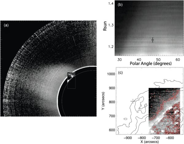
Figure 5. (a) Large-scale white-light streamer surrounding the cavity: MLSO Mk4 white-light (polarized brightness, pB) coronagraph data from 2007 August 9 (19:03:15), and (insert) EIS Fe xii 186/195 Å density–sensitive line ratio from 2007 August 9 (19:46:37). (b) August 9 daily average Mk4 r–θ pB map of NE streamer and cavity. The error bar brackets the top of the cavity, with a central top height of 1.23 ± 0.01 R☉ at 47 ± 0 5 colatitude. (c) Image showing zoomed-in EIS Fe xii 186/195 Å line ratio as a gray scale image indicating depleted density in the cavity (red contours). EIT 284 Å contours and error bar from Mk4 image are overplotted in black.
Download figure:
Standard image High-resolution image2.3. Cavity Variation with Solar Longitude
Figure 1 shows that the cavity was observed for several days, indicating a longitudinally extended structure. This can also be seen in Figure 6, which shows observations for 2007 August 9 from the EUVI instruments on the twin Solar Terrestrial Relations Observatory (STEREO)-A and B spacecraft (21:05:30 UT) bracketing SOHO EIT observations (13:12:32 UT; see Figure 7 for the relative position of the STEREO and SOHO spacecraft). These observations confirm that that the structure extended a minimum of 24° at that time since the STEREO spacecraft were separated by this amount, and the cavity is clearly visible in images from both the A and B viewpoints. Figures 8 and 9 demonstrate that the actual length is longer, with as much as 90° of longitude showing a cavity in Carrington maps, depending on the time and viewing angle of observation. Figure 1 also indicates that the height of the cavity increases and the center of the cavity at the limb moves southward with time, or decreasing longitude. This southward trend is also seen in Figures 8(a) and (c) and in Figure 9; note, however, that it is not apparent in the west limb Carrington maps. We will use our forward model to demonstrate how line-of-sight effects can explain this in Section 4.
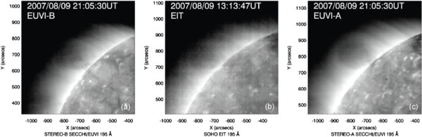
Figure 6. 195 Å images of cavity from (a) EUVI-B, (b) EIT, and (c) EUVI-A.
Download figure:
Standard image High-resolution image
Figure 7. Relative positions of STEREO-B, Earth, and STEREO-A for 21:00 UT 2007 August 9. STEREO-B: east limb Carrington longitude = −37732, heliographic latitude = 5475. Earth: east limb Carrington longitude = −27575, heliographic latitude = 6341. STEREO-A: east limb Carrington longitude = −13653, heliographic latitude = 7111.
Download figure:
Standard image High-resolution image
Figure 8. Longitude–colatitude Carrington map (CROT2060) using observations of 195 Å at the solar limb at a height of 1.1 R☉. (a) EUVI-B east limb; (b) EUVI-B west limb; (c) EUVI-A east limb; (d) EUVI-A west limb. Colored boxes show the location of the cavity observed for each view, which differ both in time and viewing angle. Arrows in (a) and (c) show longitude to the left of which the EUV cavity contrast diminished.
Download figure:
Standard image High-resolution image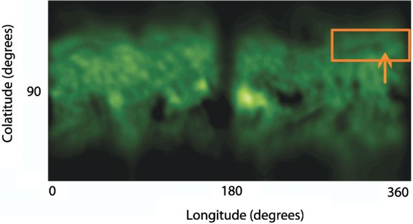
Figure 9. Longitude–colatitude Carrington map (CROT2060) using Nançay Radioheliograph  observations taken from a slice at central meridian at an assumed height of 1.025 R☉ (typical value for this frequency). A data gap occurs near map center. The cavity is seen in the orange box; the arrow indicates position to the right of which cavity visibility diminished.
Download figure:
Standard image High-resolution imageThe cavity is the limb manifestation of the filament channel observed on the solar disk (see Su et al. 2010 and references therein). This is illustrated by radio observations, which show both limb and disk. Figure 10 shows the cavity observations as seen by the Nançay Radioheliograph at  . The cavity is seen as a brightness depression on the disk and extending above the limb to match the extent of the EUV cavity (best seen in the isocontours in Figures 10(b) and (d)). Figure 11 shows the location of magnetic neutral lines and filament channels obtained from Hα. The colored rectangles indicate the Carrington longitudes where EUV and radio observations show a cavity, and illustrate that the location of the cavity overlies the neutral line of the filament channel observed in Hα, as expected. Three of the arrows show the locations where visibility of the cavity is diminished: to the left of the yellow and black arrows for the EUV observations, and to the right of the orange arrow for the radio observations. The relative visibility of the cavity may vary for these observations for several reasons. First of all, the EUV represents line-of-sight integrated limb emission, while the radio observations show emission localized to a (frequency-dependent) height at which opacity is near unity. Moreover, the observations represented by the three Carrington maps sample three different times: the east limb is observed first by STEREO-B and then by STEREO-A, and then the radio map is based on central meridian slices which are shifted in time by several days. Thus, time evolution of the cavity may affect its appearance. Finally, the Earth-view of the radio observations and the two STEREO spacecraft are from different heliolatitudes (or solar B angles), and these differences in combination with the angle and bends of the neutral line underlying the cavity can affect its visibility. We will discuss this further in Section 4 in the context of the forward modeling.
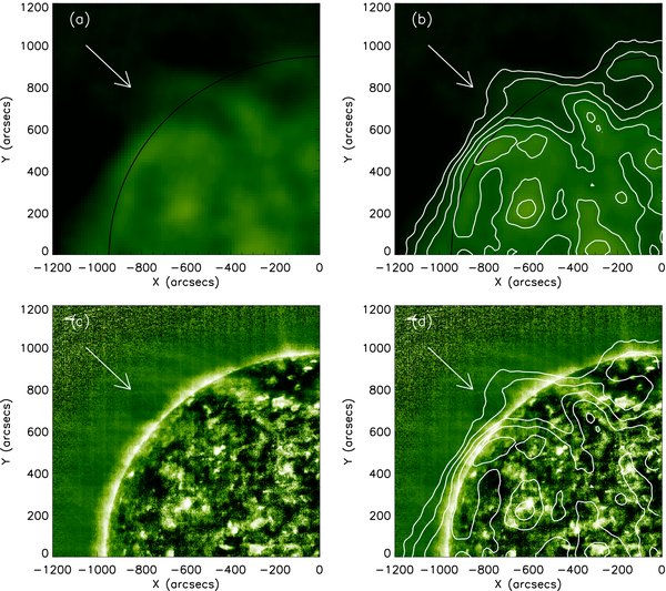
Figure 10. 2007 August 10 observations of the cavity on the NE limb (indicated by white arrow) by (a) Nançay Radioheliograph at  (11:30:30 UT) and (c) EIT 195 Å (13:13:46 UT). (b) displays radio isocontours on radio image, and (d) displays radio isocontours on EUV image. Both data sets have been enhanced for better viewing: radio data with a multi-scale filter and EIT data with a local histogram equalization. The solar limb is shown in (a) and (b) as a black line.
Download figure:
Standard image High-resolution image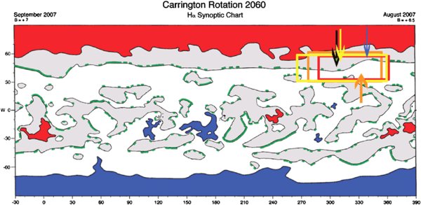
Figure 11. Carrington rotation 2060 (±30°) Hα synoptic chart (McIntosh 2003). Magnetic polarity is generally indicated by white-positive/gray-negative, with neutral lines shown as black contours. Coronal holes (identified from  ) magnetic polarity is indicated by blue-positive/red-negative. Filament channels generally lie along neutral lines, with green indicating portions where a filament was observed in Hα. The northern PCFC associated with the cavity is clearly visible at all Carrington longitudes. Colored boxes and arrows correspond to those in Figures 8 and 9 (note that the red arrow has been replaced with a black arrow for visibility); blue arrow indicates top of Λ-type shape in neutral line (see discussion in Section 4).
Download figure:
Standard image High-resolution image3. THREE-DIMENSIONAL CAVITY MORPHOLOGY
3.1. Model
We begin with a three-dimensional, global streamer density model (Gibson et al. 2003). This model builds an observationally constrained corona, beginning with a spherically symmetric background density that matches coronal hole radial density falloff as in Guhathakurta et al. (1999). We then superpose a streamer on this background, with a radial density profile as defined in Gibson et al. (1999) at the core (centered on longitude/colatitude (ϕo, θo)). Figure 12 shows schematic representations of the model with streamer parameters labeled, as viewed on the solar disk and from above. The streamer density varies in longitude–colatitude via Gaussian profiles in its (angular) length and width: the model parameter for the streamer base half-length is Slength (equivalent to  in Gibson et al. 2003), and for the half-width is Swidth (equivalent to
  in Gibson et al. 2003). The streamer half-width varies linearly in height from its photospheric value to a "current-sheet" value
  (equivalent to
  in Gibson et al. 2003) that remains fixed for all heights greater than Rcs, simulating the finite width streamer stalks surrounding current sheets extending out into the solar wind. If the streamer Gaussian has an axis parallel to the solar equator, its length runs parallel to longitude and its width to latitude. Otherwise, the length axis (which corresponds to an underlying magnetic neutral line) is defined to have an angle m to the equator. The streamer may also be non-radial with an angle α to the radial. The Gibson et al. (2003) model allows multiple streamers, but for our purposes we will just model one surrounding the cavity. Table 1 summarizes the parameters that define the model streamer.

Figure 12. Schematics illustrating the three-dimensional croissant-like cavity tunnel with elliptical cross-sections within the Gaussian streamer. Note that for simplicity, the cavity pictured has no nonradial tilt so that  . (a) View on solar disk and (b) view from above.
Download figure:
Standard image High-resolution imageTable 1. Streamer Properties
| Quantity | Parameter | Value |
|---|---|---|
| Streamer central colatitude | θo | 4555 ± 0.29 |
| Streamer central Carrington longitude | ϕo | −3033 ± 2.47 |
| Angle of streamer axis to equator | m | 895 ± 0.47 |
| Tilt of streamer height axis vs. radial | α | 0° |
| Streamer half-width at photosphere | Swidth | 15° |
| Streamer half-length at photosphere | Slength | 75° |
| Streamer current sheet height | Rcs | 2.5 R☉ |
| Streamer current sheet half-width |  |
15 |
Notes. Streamer model parameters; see Gibson et al. (2003) for details. Asterisks (*) indicate parameters that have minimal impact on cavity morphology and so are not part of the fit to cavity data. Background radial density falloff is defined by the spherically symmetric coronal hole background of Guhathakurta et al. (1999) and, for the streamer core, the model of Gibson et al. (1999).
Download table as: ASCIITypeset image
For this paper, we have modified the streamer model to allow an embedded cavity with an elliptical cross-section (see Figure 13(b)). The cavity is essentially a Gaussian-shaped tunnel oriented with its axis along the streamer axis (see Figure 12). The top of the ellipse is positioned at ( , and the length of the ellipse axis closest to radial (
 ) is measured down from the top along a line that goes through the streamer core center (r = R☉, θo, ϕo). The bottom of the ellipse is free to lie above or below r = R☉. The other ellipse axis has a length
  , defined perpendicular to
  at the ellipse center. The ellipse size decreases along the streamer length, with a Gaussian half-length Clength required to be smaller than Slength (see Figure 12(a)). The bottom of the ellipse remains at a fixed radial height along the length of the cavity tunnel, so that the top lowers as the ellipse shrinks, maintaining the aspect ratio of the ellipse (Figure 12(b)). Table 2 summarizes the model parameters defining the cavity morphology.

Figure 13. Elliptical fit to the edge of the cavity as observed in EUV. (a) Image from the EUVI-A instrument at 195 Å; (b) we show how an ellipse is fit to user-defined points along the edge of the cavity, providing the input needed to determine model parameters.
Download figure:
Standard image High-resolution imageTable 2. Cavity Properties
| Quantity | Parameter | Value |
|---|---|---|
| Cavity top radius at central Carrington |  |
1.25 R☉ ± 0.02 |
| longitude ϕo | ||
| Cavity top colatitude at ϕo |  |
4711 ± 0.70 |
| Cavity ellipse axis (nearest to radial) at ϕo |  |
0.25 R☉ ± 0.02 |
| Cavity ellipse axis (normal to Crad) at ϕo |  |
0.19 R☉ ± 0.01 |
| Cavity half-length | Clength | 345 ± 2. |
Notes. Cavity model parameters. Radial density falloff follows the streamer density falloff, but depleted by 50%.
Download table as: ASCIITypeset image
3.2. Determining Model Parameters from Observations
Figure 8 shows that the northern streamer surrounding the cavity extended more or less all the way around the Sun. As we will describe below, the central colatitude of the cavity and thus (in our model) the surrounding streamer varied with longitude, so we will fit a nonzero angle m. This requires us to model a non-axisymmetric streamer, which we center on the cavity central longitude and latitude (to be determined below). We choose values of  that ensure a streamer that is bigger than the cavity it surrounds and model a radially oriented streamer (α = 0) for simplicity. Our choices for these parameters will affect how dense the corona is at the point that a viewer's line of sight exits the cavity tunnel, and so the total line-of-sight integrated emission that is observed. However, this will only affect how dark the cavity is relative to its surrounding, and how sharp a boundary it has. As long as the density in the cavity is sufficiently reduced relative to the surrounding streamer, its morphology can be established independent from that of the streamer.
The model parameters to be determined to establish this morphology are θo, ϕo, m,  ,
,  ,
,  ,
,  , and Clength (see Tables 1 and 2). In order to fit these, we examine a sequence of EUVI images at 3 hr time resolution, August 6–12 (EUVI-A) and August 5–11 (EUVI-B). For each image, we select points along the edge of the cavity and fit an ellipse to these points (Figure 13). As we will describe below, the variation of ellipse versus Carrington longitude (equivalent to time for the rotating Sun) constrains the model parameters. Note that although we fit ellipses to both EUVI-A and EUVI-B images, we found that EUVI-B images were consistently of poorer quality, possibly because STEREO-B was over 13% further from the Sun than STEREO-A making the EUVI-B images dimmer. The parameter values quoted in the tables, and the black lines representing the fits in the figures, thus represent a fit to only EUVI-A data.
The largest source of error is the identification of the ellipse edge, because it is not uncommon for nested elliptical structures to appear in a cavity (either internal or external to the "true" cavity volume). This may be due to projection effects (e.g., a tunnel with a sloping roof might have nested internal ellipses) or to transient brightening of loop- or ellipse-like elements internal or external to the ellipse. Generally this ambiguity can be resolved by seeking the edge containing an extended (in colatitude) depletion—see, e.g., Figure 3, and by examining the cavity over an extended period of time to identify transient effects. To quantify the error involved, we have incorporated fits by multiple users (see Figure 14). Eight of the co-authors separately performed elliptical fits of the cavity versus time, resulting in a set of model parameters for each person. These parameter values were averaged for the final results and are shown along with their standard deviations in Tables 1 and 2. We identify the standard error (difference between the multi-user measured values and black line model fit, normalized to the number of free parameters) within the figure captions.
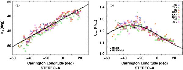
Figure 14. (a) Cavity central colatitude (θnl) at r = R☉ vs. Carrington longitude, as established by ellipse fits to the cavity as observed in EUVI-A at 195 Å. (b) Cavity top height (rctop) established by same ellipse fits also vs. Carrington longitude. Model fit is shown as black line. Different color/symbol indicates a different co-author doing the fit (identified by initials at right). The large black dot is the location of the cavity top found in white light; see Figure 5(b). Standard error for θnl is 112 and for rctop is 0.03 R☉.
Download figure:
Standard image High-resolution imageThe central colatitude of each ellipse fit at the limb (taken to correspond to the angle of the underlying neutral line, θnl) is the point where the axis closest to radial (Crad) intersects the photosphere. Figure 14(a) shows θnl versus Carrington longitude, as measured by multiple observers, with a linear fit (black line) yielding the angle m of the underlying neutral line relative to the solar equator (positive m implies a neutral line that moves northward with increasing longitude). Figure 14(b) shows how the maximum altitude of each ellipse (rctop) varies versus Carrington longitude. The peak in rctop occurs at Carrington longitude ϕo; given ϕo, θo follows from Figure 14(a).
In our ellipse fits, the colatitude of the ellipse top (θctop) was allowed to vary so that Crad did not have to be truly radial (see Figure 13(a)). We found that the difference between θctop and θnl (thus, the degree to which ellipse fits were non-radial) was small but significant (see Figure 15). Table 2 shows the central value  evaluated at ϕo for a linear fit of θctop versus Carrington longitude.
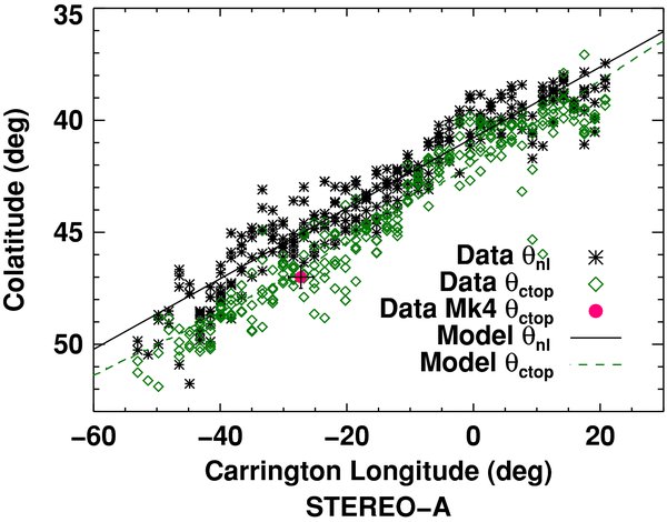
Figure 15. Cavity central colatitude θnl (black) vs. cavity top colatitude (green). The red dot shows the colatitude of the cavity top observed in white light. Standard error for θnl is 112 and for cavity top colatitude is 120.
Download figure:
Standard image High-resolution imageThe altitude of the observed cavity bottom was a free parameter in the ellipse fits. Our model assumes a single value for the position of the cavity bottom, which would be best observed at longitudes near ϕo. For longitudes between ϕo ± 15°, we find the cavity bottom lay at 1.00 R☉ ± 0.01. We therefore fixed the cavity bottom at r = R☉ for the model and calculated the distance Crad between the cavity top (rctop, θctop) and the limb (r = R☉, θnl) for each ellipse fit.
The variation of Crad versus Carrington longitude then provides a key constraint, establishing a Gaussian variation of the model cavity's near-radial axis. However, as discussed in Gibson et al. (2003), because m ≠ 0, the streamer (and so the embedded cavity) extends along a tilted "heliomagnetic longitude axis," which is fully determined now by m, θo, and ϕo (see equations for heliomagnetic longitude ϕmg in Section 4.4 of Gibson et al. 2003). The model Gaussian profile for both streamer and cavity is defined relative to this axis rather than to the Carrington longitude. We do a Gaussian fit in this coordinate system (centered on ϕmg = ϕ − ϕo) which establishes the parameters  (amplitude of Gaussian) and Clength (Gaussian half-length along heliomagnetic longitude axis). The central cavity top altitude
  also follows from
  and
and  , and the assumption that the cavity bottom is at the photosphere. Figure 14(b) shows this fit as a black line plotted versus Carrington longitude to better compare to the data. (Note that we were only able to fit about half of the modeled profile of rctop because of decreasing visibility of the cavity in the EUV images: we discuss this further in Section 4.) Figure 16 shows that, although we only used EUVI-A data to constrain the fit, it matches EUVI-B observations as well, indicating minimal time evolution of the structure.
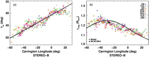
Figure 16. Points based on EUVI-B data plotted with the EUVI-A model fit (black lines) as shown in Figure 14. Standard error for θnl is 136 and for rctop is 0.04 R☉. We found the quality of data was uniformly better for EUVI-A than for EUVI-B, and so used only EUVI-A data in our fit.
Download figure:
Standard image High-resolution imageThis leaves only one remaining model parameter,  . The observed variation of ellipse-fit normal axes versus Carrington longitude somewhat overconstrains the problem, since our model requires (heliomagnetic) longitudinally invariant elliptical cross-sections. This essentially forces the same Gaussian profiles for Cnorm and Crad, with only the amplitude of the Cnorm Gaussian to be determined. This is done by fitting ϕmg versus Cnorm with a Gaussian and taking the amplitude as
  . The value of this and the other parameters thus fit are recorded in Tables 1 and 2.
4. RESULTS AND DISCUSSION
The model defined by the parameters provides a fully three-dimensional description of coronal density, which can be integrated along the line of sight to reproduce white-light pB data as was done in Gibson et al. (2003). As in that paper, the observer's position, including heliographic colatitude and longitude, can be explicitly taken into account in performing line-of-sight integration. For coronal observables other than white light, including EUV and SXR, we must also provide a temperature. For the purposes of this paper, we assume an isothermal corona of  for both cavity and streamer. EUV (or SXR) emission can then be explicitly calculated using the equation
where Int is the intensity observed in the telescope in units of DNs−1, N is the electron density, F(T,N) is a function that takes into account the atomic physics and instrument response function, and the integral is done along the line of sight, s.
Figure 17 shows the EUVI-A image of the cavity on 2007 August 9, and the forward-modeled EUV emission observed from the same Carrington longitude and heliographic latitude as the STEREO-A spacecraft at that time. For the isothermal corona, the appearance of the EUV cavity is entirely due to the density depletion that we have imposed within it. The three-dimensional morphology of the cavity does not depend on the profile we have assumed for its density, as long as it is sufficiently depleted relative to the surrounding corona that it appears in contrast to it. We have chosen a depletion value of half that of the surrounding streamer based on white-light studies, and a comparison of contour levels between Figures 17(b) and (d) indicates that this is a reasonable assumption.
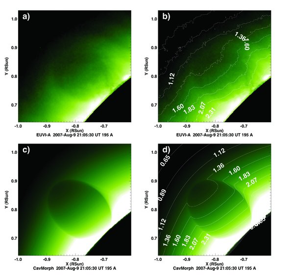
Figure 17. (a) EUVI-A image of the cavity with (b) intensity contours overlaid. (c) Forward-modeled (line-of-sight integrated) EUV emission using model density and temperature with (d) intensity contours overlaid. Contours are in units of DNs−1. See online movie for a model–data comparison of the variation of cavity location and visibility vs. time/longitude.(A color version and an animation of this figure are available in the online journal.)
Download figure:
Standard image High-resolution imageFigure 17 and the associated online movie demonstrate that the three-dimensional morphology, in particular, the size and shape of the cavity, are well matched. For example, we note the enhanced brightness of the poleward rim near the limb, which the model reproduces. This asymmetry is a projection effect discussed in Gibson et al. (2003), responsible for the "bananas" observed in white-light Carrington maps described in that paper (caused by both foreground and background material projecting to higher latitudes). The southward trend of the cavity central colatitude and the variation of its visibility with time/longitude can be seen in the online movie associated with this figure. This trend translates to a positive angle of the underlying neutral line relative to the equator, illustrated by Figure 18(a), which shows the forward-modeled EUV Carrington maps for the STEREO-A east limb viewpoint (compare to Figure 8(c), bearing in mind we are only fitting the NE streamer).

Figure 18. Forward-modeled Carrington map of (line-of-sight integrated) EUV 195 Å emission from the viewpoints of (a) STEREO-A east limb and (b) STEREO-A west limb. Maps from the STEREO-B viewpoints (not plotted) are very similar. Maps show limb emission at the height of the cavity midpoint (r = 1.125 R☉). Contours are in units of DNs−1.
Download figure:
Standard image High-resolution imageTo understand the impact of this angled neutral line on the line-of-sight integrated emission, we ran a sequence of forward models. We began with all parameters chosen as in Tables 1 and 2, except that the angle of the neutral line relative to the solar equator, m, is set to zero and (for simplicity) we set the central longitude ϕo = 180°. Figure 19(a) is the Carrington map for this model, viewed from a heliomagnetic latitude (solar B angle) of zero. The streamer and its embedded cavity for this case have a mostly symmetric emission profile, although the "banana" effect introduces a slight U-shape curvature to the streamer and a more obvious enhancement of the northern part of the streamer core (compare upper versus lower central red contours). The two vertical red lines bracket the sharply defined part of the cavity within the black contour, centered on ϕ = ϕo.
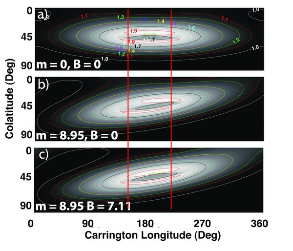
Figure 19. Carrington map (northern hemisphere) of forward-modeled (line-of-sight integrated) EUV 195 Å emission at cavity midpoint height r = 1.125 R☉. (a) Neutral line angle m and solar B angle set to zero; (b) model value of m, but still has zero B angle; (c) model value of m, and the solar B angle as seen from the viewpoint of STEREO-A during the time of the cavity observations. Note we have shifted to ϕo = 180 to center the structure for easier viewing. Contours in (a) are in units of DNs−1: to avoid cluttering the plot we have not plotted them in (b) and (c), but note that the values for the various color contours are the same in (a)–(c).
Download figure:
Standard image High-resolution image
In the middle image, we run our forward model with the neutral line angle set to the model value m = 895, but maintain a heliomagnetic latitude of zero. As discussed in Wiik et al. (1994), the optimal viewing angle for a cavity is along an underlying neutral line angled at exactly the solar disk polar angle corresponding to its central limb latitude. However, for line-of-sight integrated (optically thin) EUV emission, this optimal angle switches sign for frontside versus backside material. In Figure 19(b), the neutral line angle m tilts the cavity axis further away from the solar disk polar angle for the foreground, but more along the solar disk polar angle for the background. When the cavity first becomes visible, more of its length is in the background, and so the neutral line angle improves the viewing somewhat. As we pass the cavity central Carrington longitude ϕo, however, the neutral line angle works against visibility. The effect of this is seen in Figure 19(b), in which the central black contour has shrunk and shifted to the right (greater Carrington longitude = earlier times).
There is one more angle that needs to be taken into consideration: the heliomagnetic latitude of the observer. Figure 19(c) illustrates that, for the STEREO-A viewing position (east limb), the solar B angle nearly compensates for the neutral line angle m. The result is a forward-modeled streamer-cavity structure that is largely symmetric in heliomagnetic latitude/longitude, and that is more distinctly visible than the Figure 19(b) case. The central black contour is still shifted a little to the right as compared to Figure 19(a), but otherwise has a very similar size and shape.
We now return to Figure 18, which shows our best-fit forward-modeled EUVI-A emission for both for the east and west limb. Figures 18(a) and (b) can be directly compared to Figures 8(c) and (d), and it provides an explanation for the lack of cavity visibility at the west limb. At the west limb, the m angle acts in the opposite way from the east limb (foreground material tilted down, background material tilted up), and the positive solar B angle decreases, rather than increases cavity visibility. Gibson et al. (2003) used a related argument to explain the east–west asymmetry in Carrington maps where northern streamers slanted up and to the right for east limb maps, and up and to the left for west limb maps when viewed from a positive solar B angle (see also discussion in Wang et al. 1997). This can in fact be seen in the observations shown in Figure 8, and in the forward model fit of Figure 18, where the west limb cavity is not only diminished but is angled up and to the left relative to the east limb cavity.
We were only able to constrain our fit with measurements from ellipses to just past the Gaussian midpoint, because, as Figure 8(c) shows, the cavity contrast was lost below around Carrington longitude of 300° (yellow/black arrows). However, despite the loss of contrast, a cavity is observationally distinguishable in Figure 8(c) down to Carrington longitudes of nearly 270° (as indicated by the yellow box). This longitudinal extent is captured by the full Gaussian of our forward model (Figure 19(c)). The loss of cavity contrast may be due to departures from a linear m angle of the underlying neutral line. Figure 11 indicates that the slope of this neutral line flattens out close to where the EUV cavity dims (yellow/black arrows); at this point the slope's effect on foreground material would be working against visibility, and we would also lose the benefit of that slope for the background material. Conversely, the Λ-shaped kink in the neutral line shown by the blue arrow would improve visibility, at least for line-of-sight integrated EUV, as there would be less of a harmful slope in the foreground, and more of a helpful slope in the foreground. Indeed, the blue arrow points to a Carrington longitude where the cavity was particularly visible at the east limb.
5. CONCLUSIONS
The analysis presented here represents the first step of a process to establish a three-dimensional distribution of density and temperature in and around the 2007 August coronal prominence cavity. The broad range of observations we have employed, including wavelength and viewpoint coverage, has allowed us to tightly constrain the three-dimensional morphology of this cavity. This sort of analysis complements EUV tomographic reconstructions (Vasquez et al. 2009, 2010), which do not require a predetermined model form for the cavity morphology, but which can only provide information for radial heights possessing significant EUV signal. Our limb-view ellipse-fitting technique allows us to fit the full three-dimensional cavity morphology, with the curvature of the cavity boundary providing the clue to where the cavity top lies. The comparison with white-light data (e.g., the Mk4 data points in Figures 14(b) and 15) allows verification of this extrapolation of shape. In general, the comparison of forward-modeled observables to the data justifies the form of our morphological model.
Perhaps the greatest strength of a forward-modeling approach is that it is possible to consider how a given three-dimensional structure like the cavity may appear from different vantage points and for different observables. The sensitivity of cavity visibility to viewing angle is considerable: changes of a few degrees in neutral line orientation and/or observer's solar B angle are enough to obscure it. For example, we have demonstrated with the model why a cavity may be clearly visible on one limb and not the other, as the solar B angle can act to increase cavity visibility on one limb, but decrease visibility on the opposite limb. It is of course possible that evolution of the structure over the 2 weeks between east and west limb viewing may also play a role in the differences. However, the fact that our east limb model fit to EUVI-A data reproduced EUVI-B data reasonably well (Figure 16) is evidence that the cavity did not change greatly during the multiple days we observed it.
Our analytic morphological model is also needed to properly consider line-of-sight projection effects on the unique spectroscopic data from the IHY observing campaign. Such projection effects may arise both because of density and temperature gradients in the cavity and because of the intrusion of bright streamer material along the line of sight. Our campaign obtained temperature and density-sensitive diagnostic data from Hinode EIS and SOHO CDS, with long exposure time and broad spectral coverage designed for cavity analysis. These data were taken on August 9, which was the day the cavity was most clearly visible from Earth. Although we have established already that the cavity has a relatively low density compared to the surrounding streamer, the quantification of its density and temperature remain future projects of relevance to understanding the MHD state of the prominence cavity (D. J. Schmit et al. 2011, in preparation; T. A. Kucera et al. 2011, in preparation).
The three-dimensional structure of the magnetic field in the prominence and surrounding cavity controls that MHD state in the magnetically dominated corona and remains an open question (see e.g., van Ballegooijen & Cranmer 2010 and references therein). New developments in coronal magnetometry (Lin et al. 2004; Tomczyk et al. 2008) have opened possibilities for forward magnetic modeling. Indeed, efforts are underway to compare Coronal Multichannel Polarimeter (CoMP) observations of a cavity in 2005 to polarimetric observables determined from an MHD application of our forward codes (J. Dove et al. 2011, in preparation). In general, the techniques and software we have developed for fitting cavity observations and translating time sequences to a three-dimensional morphological model represents a considerable asset for a broad range of future analyses of cavities. It will be interesting to use them to study how cavity properties may vary with wavelength, size, latitude, and time of solar cycle, as well as how they may evolve just prior to an eruption.
We thank the International Space Science Institute (ISSI), which funded a Working Group on Coronal Cavities involving many of the co-authors. We thank Alice Lecinski for internal HAO review, Joan Burkepile for assistance with the Mk4 data, and Arnaud Thernisien for assistance with the STEREO Carrington maps. A.C.S. and T.A.K. were supported by the NASA SHP program. SOHO is a project of international collaboration between ESA and NASA. Hinode is a Japanese mission developed and launched by ISAS/JAXA, with NAOJ as domestic partner and NASA and STFC (UK) as international partners. It is operated by these agencies in cooperation with ESA and NSC (Norway). The STEREO/SECCHI data used here are produced by an international consortium of the Naval Research Laboratory (USA), Lockheed Martin Solar and Astrophysics Lab (USA), NASA Goddard Space Flight Center (USA) Rutherford Appleton Laboratory (UK), University of Birmingham (UK), Max-Planck-Institut fr Sonnensystemforschung (Germany), Centre Spatiale de Liege (Belgium), Institut d'Optique Thorique et Applique (France), and Institut d'Astrophysique Spatiale (France). The National Center for Atmospheric Research is supported by the National Science Foundation.