


ABSTRACT
2008 marked the beginning of sunspot cycle 24 in the inner heliosphere. Intensities of galactic hydrogen and helium measured by the Voyagers in 2008 were the highest ever recorded and believed to be approaching the interstellar values. We investigate transport of galactic cosmic ray (GCR) protons in the three-dimensional, asymmetric heliosphere, including the inner heliosheath region, by tracking stochastic phase-space trajectories of Parker equation under steady plasma background conditions. The latter is calculated from a three-dimensional MHD model of the global heliosphere that takes into account the effect of neutral hydrogen atoms. The model is applied to quiet solar wind (SW) conditions appropriate for the 2008–2009 solar minimum. Model-derived cosmic-ray spectra and radial gradients are reviewed in the context of Voyager observations in the heliosheath. It is shown that the heliosheath is an important modulation barrier for lower energy ions. Radial cosmic-ray gradients in the heliosheath are expected to be small in the directions of the Voyagers (1.5%–1.8% per AU at 180 MeV). In our model the termination shock does not accelerate GCR ions very efficiently, and their intensities in the heliosheath never exceed interstellar values. Analysis of cosmic-ray residence times in different parts in the heliosphere shows that, prior to their detection, ions spend 3–6 times longer transiting the heliosheath and the heliotail than they spend in the supersonic SW.
Export citation and abstract BibTeX RIS
1. INTRODUCTION
The year 2008 and the early 2009 saw unusually low levels of solar activity (ftp://ftp.ngdc.noaa.gov/STP/SOLAR_DATA/SUNSPOT_NUMBERS). Sunspot cycle 24 has begun in the second half of 2008, although it is not yet known whether the solar minimum has been reached at the time of this writing (D. H. Hathaway 2009, private communication). Intensities of galactic cosmic rays (GCRs) were still on the increase at the Earth in early 2009 as seen from the ACE data (http://www.srl.caltech.edu/ace/asc/level2/lvldata_cris.html), indicating that the minimum modulation level has not been reached yet. Generally speaking, drift along the neutral sheet is the principal mechanism that brings positive ions into the inner heliosphere during negative solar minima (Jokipii & Kopriva 1979; Kota & Jokipii 1983; Lopate & Simpson 1991; McDonald et al. 1992; Jokipii et al. 1993; Webber & Lockwood 1997), with cross-field diffusion playing a more prominent role within a few AU from the Sun (Kota & Jokipii 1995; Potgieter 2000; Ferreira & Potgieter 2004; Parhi et al. 2004). Seen on the global scale, positively charged ions enter along the sheet and leave at high latitudes, where the drift velocity is away from the Sun. Perpendicular diffusion acts to spread the energetic particles to high latitudes reducing latitudinal gradients in the inner heliosphere (Heber et al. 2008).
Whereas this well-established concept appears to work well in the solar wind (SW), the situation in the heliosheath is more uncertain. The heliosphere is a topologically complex structure produced by the interaction between the SW plasma and the partially ionized flow of the circum-heliospheric interstellar medium (CHISM). With the advent of MHD models of the outer heliosphere the global structure of the region and the geometry of the magnetic field in the heliosheath began to emerge. The supersonic SW is not directly affected by the charged component of the interstellar flow, which is diverted around the heliopause (HP). Interstellar neutral atoms are unimpeded by the solar magnetic field and can penetrate to within a few AU of the Sun before they become ionized. In charge exchange collisions neutral atoms deprive the SW of its bulk momentum reducing the SW velocity by ∼15% near the termination shock (TS; Richardson et al. 2008b), but otherwise do little to break the azimuthal symmetry of the SW flow. Conversely, the subsonic heliosheath is an asymmetric structure, being directly affected by the variations of the interstellar plasma flow and of the pressure of the interstellar magnetic field on the surface of the HP (Washimi & Tanaka 1996; Linde et al. 1998; Pogorelov & Matsuda 1998; Ratkiewicz et al. 1998; Izmodenov et al. 2005; Opher et al. 2006; Pogorelov et al. 2007).
GCR activity in the outer heliosphere is monitored by the two Voyager space probes. Voyager 1 (V1) left the supersonic SW region and entered the heliosheath in December of 2004 (Decker et al. 2005; Stone et al. 2005; Burlaga et al. 2005), and Voyager 2 (V2) followed in September of 2007 (Richardson et al. 2008a; Decker et al. 2008; Burlaga et al. 2008; Stone et al. 2008). By the start of 2009 V1 and V2 have accumulated 4 and 1.5 years worth of GCR observations in the heliosheath, respectively. From the year 2005 on GCR ion intensities measured by both spacecraft were rising steadily after reaching a minimum at the end of 2004 (Webber et al. 2008). The apparent time-dependent radial gradient of 180 MeV protons in 2006–2008 was about 7%/AU (http://voyager.gsfc.nasa.gov/heliopause/heliopause/archive_26d.html). This very large "dynamic" gradient was a product of the declining levels of heliospheric modulation, rather than being a signature of a large positive "static" radial gradient in the heliosheath (McDonald et al. 2007). The latter can be deduced from the difference between intensities at V1 and V2 that are radially separated by 20 AU. If latitudinal gradients are taken to be small, this yields a much more modest ∼1% per AU gradient in the heliosheath at the same energy. At higher rigidities the gradient is even smaller, ∼0.2% per AU for 330 MeV/n GCR He (compare Stone et al. 2008; Webber et al. 2008).
Global three-dimensional heliospheric models have now reached a level of maturity where it becomes possible to use them as background to study the transport of energetic particles in the entire volume of space controlled by the SW plasma. The heliosheath region has long been recognized as a modulation barrier capable of filtering the GCRs incident from the CHISM (Webber & Lockwood 1987; Jokipii et al. 1993; Langner et al. 2003; Caballero–Lopez et al. 2004). Global kinetic models of GCR transport in this region based on model-calculated, rather than prescribed, plasma and magnetic field backgrounds were developed by Florinski et al. (2003), Ferreira & Scherer (2004), and Ferreira & Scherer (2006). These models were axially symmetric about the direction of the interstellar flow vector. Florinski et al. (2003) emphasized the role of the heliosheath as a barrier preventing lower-energy cosmic rays from reaching the inner heliosphere. In their model magnetic field in the heliosheath was strongly amplified near the stagnation point resulting in a "modulation wall" lining the inside of the HP. Significant GCR attenuation was predicted within the wall, but otherwise radial gradients in the heliosheath were expected to be small.
Lacking the fully three-dimensional magnetic field, axisymmetric models ultimately miss some of the physics relevant to cosmic-ray transport. The heliosphere is an essentially three-dimensional structure, without well-defined planes or axes of symmetry. The HP tends to become elongated in the direction along the CHISM magnetic field and compressed in the perpendicular direction (e.g., Linde et al. 1998; Pogorelov et al. 2004). The HP may be tilted in the meridional plane depending on the angle between the flow speed and the magnetic field B in the CHISM (Ratkiewicz et al. 1998; Pogorelov et al. 2004; Izmodenov et al. 2005). This naturally leads to an asymmetric plasma flow in the heliosheath region. Likewise, the TS is asymmetric, due to (1) latitudinal variation of the SW dynamic pressure, leading to an ecliptic-to-pole asymmetry (Nerney & Suess 1995; Pauls & Zank 1996; Barnes 1998; Washimi & Tanaka 2001), and (2) due to nonuniform confining pressure in the heliosheath and the tail, manifested in a simple nose-tail asymmetry (Suess et al. 1987; Baranov & Malama 1993; Pauls et al. 1995; Fahr et al. 2000), and in a more complicated distortion of the shape of the TS (e.g., Opher et al. 2006; Pogorelov et al. 2008). Axisymmetric models are unable to resolve these asymmetries, nor can they include a realistic profile of the neutral sheet in the heliosheath. Finally, treatment of the heliospheric magnetic field in such models is necessarily kinematic because the j × B force orthogonal to the simulation plane cannot be accommodated. This can overestimate the field strength near the stagnation point, where the plasma speed u ≃ 0. Evidently, the shape of the boundaries and the volume of space available to GCRs are affected, and so are the drift patterns and the diffusion coefficients.
Recognizing the drawbacks of the two-dimensional approach Ball et al. (2005) developed a three-dimensional model based on the stochastic transport theory. Florinski & Pogorelov (2008) considered a similar three-dimensional problem using a grid-based approach to solve Parker's transport equation. Both techniques have their advantages and drawbacks, which are discussed in Section 3. Implicit grid models yield a cosmic-ray distribution at every point in the simulation domain, but are very computationally intensive. The output from a stochastic model is intensity at one specific point in phase space. Because of their relative simplicity and low computational demand stochastic codes are particularly useful for exploring the parameter space of the problem. Here, we report results from a new four-dimensional (three-dimensional+momentum) model of GCR transport in the global heliosphere, based on the stochastic trajectory approach. Preliminary results from this model were reported in Florinski (2009). Our particle transport model essentially follows from first principles, with drifts and diffusion coefficients derived from theoretical models. A simpler phenomenological approach is adopted to describe turbulence transport throughout the heliosphere. We focus on GCR transport in the heliosheath during negative solar minimum conditions. Proton spectra recently measured in the heliosheath are compared with our model calculations. We also discuss radial gradients in the heliosheath in the context of Voyager observations. Finally, we investigate the residence times of galactic protons in the different parts of the heliosphere, including the supersonic SW, the heliosheath, and the heliotail. It is shown that whereas the heliosheath does affect the transport of galactic particles with energies from below 100 MeV to ∼1 GeV, its role as a modulation barrier during solar minima is not as pronounced in comparison to axisymmetric heliospheric model predictions.
2. PLASMA AND TURBULENCE BACKGROUNDS
All results reported here correspond to a heliospheric configuration appropriate for periods of time near an A < 0 solar minimum. To obtain the velocity and magnetic field backgrounds we use an MHD model coupled to a hydrodynamic neutral fluid model (Pogorelov et al. 2006). This approach was shown to yield plasma parameters consistent with those obtained with more sophisticated kinetic neutral codes (Heerikhuisen et al. 2006). We assume that SW conditions change slowly and the background can thus be regarded as stationary.
The inner boundary of the simulations is placed at rmin = 10 AU, where a latitude-dependent SW inflow is specified. Fast coronal hole wind with inflow velocity of 800 km s−1 is confined to latitudes above 30°, whereas slow SW with velocity of 400 km s−1 fills the remaining space (all values given are at 1 AU, they are extended to the inflow boundary using the standard SW solution). SW density is 2.7 cm−3 and 7.0 cm−3 at high and low latitudes, respectively. These values are representative of solar minimum conditions as measured by Ulysses (McComas et al. 2000). The magnetic field is of a Parker type with a radial component of 28 μG (2.8 nT) and a thin neutral sheet separating oppositely directed fields in the northern and the southern hemispheres. Because we assume no dipole tilt, the sheet is essentially flat in the SW but flips to the north in the heliosheath. The location of the inner boundary and the flat neutral sheet are the limitations of the plasma background model (for a more complete description of the model see Pogorelov 2006). Placing the boundary closer to the Sun or trying to resolve the oscillating tilted neutral sheet would incur a severe penalty in computation time. Results with an oscillating neutral sheet were recently reported by Pogorelov et al. (2009). Work is underway to adapt their model to cosmic-ray transport.
The external boundary is located at rmax = 1000 AU. For the CHISM flow we assume plasma density of 0.05 cm−3, velocity V∞ = 26.4 km s−1, and temperature of 6527 K. The tilt of the ecliptic plane relative to the CHISM velocity vector is neglected here (see Pogorelov et al. 2007). A magnetic field B∞ = 1.5 μG (0.15 nT) orthogonal to V∞ is specified in the CHISM. The field is tilted by 60° relative to the ecliptic plane and points northward. Thus, the plane between B and u (the so-called BV-plane) is nearly parallel to the hydrogen deflection plane in Solar and Heliospheric Observatory (SOHO) observations (Lallement et al. 2005). The model includes interstellar hydrogen atoms as a single neutral population. This population is assumed to be in thermal equilibrium with the plasma at the external inflow and has a density of 0.15 cm−3. The two fluids are coupled via charge exchange, and the computed three-dimensional structure of the heliospheric interface is strongly influenced by this interaction (Pogorelov et al. 2006, 2007).
Figure 1 is a three-dimensional cutout view of the heliosphere showing the magnitude of |B|. This simulation is based on a spherical grid with 252 × 154 × 138 cells in the r, θ, and φ directions, respectively. The cell size in the radial direction was about 0.6 AU at the inner boundary increasing to 1.4 AU at the TS. Note the coordinate axes direction shown in the upper right corner (Ox is along the inflow direction, Oz points toward the heliospheric north, and Oy completes the right-handed coordinate system). The shapes of the TS and the HP are shown with black lines. Note the shock elongation over the poles and in the tailward direction. The boundary (difference in color) between heliospheric and interstellar plasmas is less distinct near the nose of the HP, but can be traced farther along the flanks. The interstellar magnetic field is draped around the nose of the HP, and is generally stronger than its interplanetary counterpart on the heliosheath side. The heliomagnetic field, while much weaker in most of the outer heliosphere, is amplified on approach to the HP close to the stagnation line, where it is comparable in magnitude with the interstellar field (a few μG). Inside the TS B is stronger in the slow SW at low latitudes. The neutral sheet is seen separating oppositely directed fields in the northern and the southern hemispheres. After crossing the TS, the neutral sheet is carried northward by the flow of heliosheath plasma. The bending of the neutral sheet occurs because of an interaction between the magnetic fields across the HP. The direction of bending (north vs. south) is somewhat sensitive to the direction of the magnetic field in the CHISM (Pogorelov et al. 2006). Unlike the axisymmetric MHD model used by us earlier (Florinski et al. 2003), this fully three-dimensional simulation features asymmetric TS and heliosheath owing to a tilt of the interstellar magnetic field relative to the ecliptic plane.
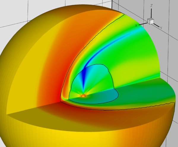
Figure 1. Three-dimensional cutout view showing the magnetic field magnitude |B|, on a logarithmic scale, in the meridional (xz) and solar equatorial (xy) planes. The orientation of the main axes is shown in the upper right corner. The black lines trace the shapes of the TS and the HP. The interplanetary magnetic field, normally much weaker than the interstellar field, is compressed near the HP forming the magnetic wall. Note the neutral sheet flip to the north in the heliosheath.
Download figure:
Standard image High-resolution imageEnergetic particles are scattered by turbulent fluctuations, and a certain amount of information about turbulent intensity in the heliosphere is therefore required. We assume that the turbulence content of the heliospheric plasma can be described with only two basic parameters: the mean square turbulent magnetic field intensity, 〈δB2〉, and the "bendover length" lb that marks the transition between the energy-containing and the inertial regions of the turbulent power spectrum (see Zank et al. 1998). lb is simply related to the correlation length of the turbulence. The power spectrum is a combination of a flat energy range and a k−5/3 Kolmogorov inertial range, the transition between the two occurring at k = 2π/lb. In our earlier work (Florinski & Zank 2006) the turbulent background of the SW was modeled on the turbulence transport theory developed by the Bartol group (Zhou & Matthaeus 1990; Zank et al. 1996; Matthaeus et al. 1999). Here, we adopt a somewhat simpler approach by using the results of Breech et al. (2008). According to their calculations the intensity of turbulent fluctuations scales approximately as 〈δB2〉 ∼ ρ beyond 10 AU, which is the inner boundary in our simulations (ρ is the SW plasma density). This behavior is sometimes referred to as the Jokipii–Kota regime (Jokipii & Kota 1989). Consequently, we assume that
at all latitudes, where 〈δB2〉10 is the turbulent field at 10 AU in the ecliptic plane, and ρ10 is the representative SW density at this distance, corresponding to a number density of 0.05 cm−3. The assumption of latitudinal independence in the outer heliosphere is roughly consistent with Breech et al. (2008), except that the enhancement in the transition region between the slow and the fast wind is not included here. The bendover length varies only weakly and is taken here to be a constant between the inner boundary and the TS. The actual numerical values of 〈δB2〉10 and lb are listed in Section 3.
A turbulence transport theory for the heliosheath has not been developed yet, largely due to a paucity of observational data. Following Florinski & Zank (2006) we assume that 〈δB2〉 increases by a factor equal to a square of the shock compression ratio upon crossing the TS and further that 〈δB2〉 ∼ B2 along the streamlines extending from the TS into the heliosheath and the heliotail. The turbulent ratio, which serves as a measure of the plasma turbulent content, is calculated as 〈δB2〉/B2tot, where B2tot = B2MHD + 〈δB2〉, with BMHD being the magnitude of the magnetic field from the MHD model. Because the latter necessarily does not include the fluctuating component, the above correction is necessary to ensure that the turbulent ratio is less than 1. The ratio is typically higher at high latitudes and inside the current sheet, where BMHD is small.
3. STOCHASTIC TRANSPORT MODEL
GCR ions have large energies and their anisotropies are accordingly small. In this limit it is sufficient to consider the pitch-angle-averaged phase-space density f(r, p), which is a function of spatial position and the magnitude of momentum p. Transport is modeled with Parker's equation (Parker 1965; Gleeson & Axford 1967) that can be written as
where u is the plasma velocity. The drift velocity vd for an isotropic distribution of particles is
where w is the particle speed and e its charge.
The diffusion tensor κij = κ⊥δij + (κ∥ − κ⊥)bibj, where b = B/B, is a function of the particle's momentum and of the turbulent fluctuation energy available to scatter the particles. Once the turbulent content at the inflow is fixed, the transport model is complete. Parallel mean free path is calculated from the quasi-linear expression (similar to Florinski et al. 2003, their Equation (18)). We take the intensity of slab modes to be 10% of the total, the remaining being two-dimensional turbulence (Bieber et al. 1996). For the perpendicular diffusion we use two different expressions: (1) a constant fraction based on the turbulent ratio, hereinafter referred to as the LZP model (le Roux et al. 1999) with
where a is a constant of the order of 0.01–0.1, and (2) the nonlinear guiding center (NLGC) expression (Matthaeus et al. 2003; Zank et al. 2004; Shalchi et al. 2004)
where b is a constant of the order of 1. Both models assume that turbulence is axially symmetric with respect to B. In the LZP and the NLGC models we used 〈δB2〉10 = 3 × 10⁻¹² G2 and 5 × 10⁻¹² G2, respectively. The bendover length lb was 0.05 AU in both the SW and the heliosheath in the LZP case. In the NLGC model lb was 0.1 AU in the SW decreasing to 0.033 AU beyond the TS. These parameters yielded the best fit to the observed GCR proton intensities measured at 1 AU and at ∼95 AU. We used a fixed value b = 1.1, which again yielded results that were most consistent with the observations. The only free parameter available for us to vary was a in the LZP model (Section 4.3 discusses the parametric dependence of GCR fluxes on κ⊥/κ∥). In most of the simulations we assumed a = 0.03.
Figure 2 illustrates the radial dependence of the parallel and the perpendicular diffusive mean free paths along the direction 10° north in the xz (meridional) plane. Of note is a decrease of λ∥ and λ⊥ across the TS with a further slow reduction in the heliosheath toward the HP. A dip in λ∥ near the HP occurs as the radial ray crosses the neutral sheet. Evidently, in the LZP model λ⊥ closely follows λ∥, whereas it varies less in the NLGC model due to a weaker λ1/3∥ dependence. The ratios λ⊥/λ∥ used here are consistent with the values quoted in the literature (e.g., Zank et al. 2004).
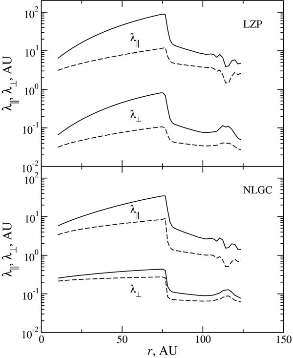
Figure 2. Parallel and perpendicular diffusive mean free paths in the meridional plane along the direction 10° north in the LZP (top panel) and the NLGC (bottom panel) models. Solid lines are for 1 GeV protons and dashed lines are for 100 MeV protons.
Download figure:
Standard image High-resolution imageParker's transport equation may be inverted numerically using one of the two broad classes of solution techniques termed here "field" models and "particle" models. In the first approach, the phase-space distribution f(r, p) is treated as a four-dimensional scalar field, discretized on an appropriate grid. In view of very high stiffness of the parabolic transport equation, a field solver is required to be of an implicit type, whereby every grid cell is causally connected to all other cells in the grid. "Field" models traditionally have been more popular in this field (e.g., Jokipii & Kopriva 1979; Potgieter & Moraal 1985; Jokipii et al. 1993). Multiple dimensions were addressed with Alternate Direction Implicit (ADI) schemes which split the original multidimensional problem into several quasi-one-dimensional problems. Florinski & Pogorelov (2008) argued that ADI methods, while adequate to use on prescribed magnetic and diffusion fields, are not reliable enough to handle model-calculated three-dimensional magnetic fields that produce a high degree of anisotropy and nonuniformity in cosmic-ray transport coefficients. ADI techniques tend to fail in these situations because they treat mixed second derivatives in the parabolic transport equation explicitly. An alternative technique is to use a fully implicit multidimensional code. The objective is then to invert a large sparse matrix, typically containing millions of equations. Florinski & Pogorelov (2008) demonstrated a solution method based on a preconditioned Krylov subspace solver. Their approach resulted in a more robust numerical scheme, but at the same time was quite computationally intensive requiring a supercomputer and thousands of CPU-hours for a problem of any reasonable size.
The "particle" approach is based on a statistical treatment of the transport equation. Here, the distribution f at a given point in phase space is constructed by averaging over the exit points of a large number of phase trajectories of the transport equation. Each trajectory describes one realization of particle's guiding center motion (Zhang 1999). Trajectories contain a deterministic component (drift, convection, and adiabatic energy change) and a probabilistic part (spatial and/or momentum diffusion). This approach exploits a mathematical equivalence of a parabolic partial differential equation, such as Parker's equation, and a system of stochastic differential equations (SDEs) of the Ito type. Parker's equation describes the evolution of the probability density for a particle to be found at a point (r, p) in phase space. An SDE is a first-order ordinary differential equation containing a random rapidly fluctuating term. For a systematic discussion of the SDE theory and its application to diffusive transport see Gardiner (1985). Jokipii & Owens (1975) first applied a stochastic method to cosmic-ray transport in the SW. Subsequent works employing SDEs in this field include MacKinnon & Craig (1991), Krülls & Achterberg (1994), Chalov et al. (1995), and Zhang (1999).
Here, we follow closely the works of Zhang (1999) and Ball et al. (2005) by integrating stochastic particle trajectories backward in time until they reach the external boundary of the simulation. To this end Parker's equation must be rewritten as a backward Fokker–Planck equation (Gardiner 1985), viz.,
Note that the divergence of the diffusion tensor in Equation (6) may be written under the assumption that κ⊥ ≪ κ∥ as

The deterministic part is readily integrated using characteristics
The probabilistic component is given by

where AikAkj = 2κij and Wi(t) is a multidimensional Wiener (random walk) process such that  . It is more convenient to rewrite the diffusive part in a local coordinate system where the diffusion tensor is diagonal. Let us take the z' axis along B and write the transport equation containing diffusive terms only as
where cylindrical coordinates (r, φ, z'), local to the particle's position, were used. The equivalent SDE formulation is


Here, Z and R are normalized displacements along the mean field and in the plane perpendicular to the mean field, respectively, and 0 ⩽ nr, nz, nφ ⩽ 1 are uniformly distributed random numbers. Differential displacement probabilities are normally distributed with mean 0 and variance 1/2
The random numbers nr and nz correspond to cumulative probabilities obtained by integrating Equations (15) and (16), viz.,
Z and R themselves are obtained by inverting these distributions to obtain

where erf−1 is the inverse error function, and

To find the displacements in the global (solar) rest frame the paths (12)–(14) are projected onto the main coordinate axes. If c is a unit vector in the direction of perpendicular transport, then probabilistic displacements may be written as

The total displacements are given by dxi = dxdeti + dxproi.
We treat the inner boundary r = rmin as a reflecting barrier for cosmic-ray particles. We also assume that the space beyond the HP is uniformly filled with pristine interstellar distribution f∞(p). To calculate f(r, p) a large number (typically tens of thousands) particle trajectories are integrated backward in time using Equations (8), (9), and (21) until the trajectory intersects the HP. Time steps are calculated from a local CFL condition. The solution is an average over all exit points
where f∞ is the interstellar GCR spectrum (see below), pend,i is the momentum of the ith particle at the end of its trajectory, and N is the total number of particles in a simulation.
4. GCR TRANSPORT IN THE OUTER HELIOSPHERE
This section contains the principal results from the model. We discuss spectral features and radial profiles, focusing especially on the heliosheath region. We also show how intensities depend on the ratio κ⊥/κ∥. Heliospheric residence times are discussed in Section 5 below.
4.1. Spectral Information
Figure 3 shows GCR proton differential intensity J = fp2 calculated at two locations inside the heliosphere for A < 0 solar minimum conditions. The CHISM proton spectrum f∞, prescribed at the boundary, was taken from Webber & Higbie (2009) (black line in Figure 3). Spectra at other spatial locations inside the heliosphere were produced by running time-backward simulations of 200,000 stochastic trajectories each and binning the results into 50 momentum bins spaced logarithmically between 30 MeV and 5 GeV. Shown are two sets of spectra calculated using the LZP model (solid lines) and the NLGC model (dashed lines). We show 11 AU (1 AU past the inner boundary) spectra as representative of those in the inner heliosphere (shown with blue color). Heliospheric spectra have a classic modulated shape with a broad maximum appearing at a few hundred MeV. With decreasing energy a progressively larger fraction of the particle flux is derived from higher energy protons cooled by the expanding SW, the spectrum thus asymptotically approaching the slope J ∼ T at low energies in the inner heliosphere, visible in both spectra at 11 AU.

Figure 3. Proton spectra during the A < 0 solar minimum at 11 AU in the ecliptic and at 95 AU along the direction 35° north in the meridional plane (along the V1 trajectory). The black line is the pristine CHISM spectrum used as the boundary condition (Webber & Higbie 2009). 11 AU calculated spectra are shown in blue, and 95 AU spectra in red. Solid lines are LZP results and dashed lines are NLGC results. 95 AU spectra are compared with 2008 V1 data (squares; Webber et al. 2008). Also shown is a proton spectrum measured at the Earth in 2007 by the Pamela experiment (diamonds; Casolino et al. 2009).
Download figure:
Standard image High-resolution imageSince no GCR observations at 11 AU are available, we use 1 AU observations to do a consistency check. Plotted in Figure 3 are observations made with Pamela in Earth's orbit during 2007 (shown with diamonds in this figure; Casolino et al. 2009). The LZP and the NLGC models are mostly consistent at high energies, but differ in their predictions at lower energies. This is not necessarily a reason to prefer one model over the other since intensities at 11 AU are likely to be higher than those at 1 AU. Also shown in Figure 3 are spectra calculated for the approximate direction of V1 travel at a latitude 35° north at a radial distance of 95 AU. Here, the two diffusion models give similar predictions that are generally consistent with V1 observations from 2008 (shown with squares; Webber et al. 2008). The fit is not as good at the low end of the spectrum in the NLGC model. Note that the calculated heliosheath spectra never exceed interstellar intensity. This contradicts the results of Florinski et al. (2003) and Ferreira & Scherer (2006) that show an excess in heliosheath intensity at high (GeV) energies. The difference is related to a lack of significant re-acceleration of high-energy GCRs by the TS in our model, see Section 4.2 below.
Both our diffusion models predict strong attenuation of GCR fluxes by the heliosheath, which is qualitatively in agreement with our earlier two-dimensional results (Florinski et al. 2003). Figure 3 shows that intensities at 200 MeV at 95 AU are at 50% their interstellar value in both cases. This does not mean that half of all incoming 200 MeV protons are filtered by the heliosheath: the percentage rate could be higher, with the missing population made up by higher energy ions cooled down in the SW and transported outward to the TS. This possibility is discussed in more detail in Section 5 (see also Ball et al. 2005).
The model spectral fits to the observations are, of course, not perfect. It would be possible to obtain better fits by adjusting relevant parameters or selecting a prescribed diffusion model. That, however, would go against the spirit of this work, which is to investigate GCR transport using magnetic field and turbulence data directly from the model of the plasma background and relying on theoretical predictions for the diffusion coefficients. The degree of similarity between the model and the observations is actually remarkable given the complexity of the underlying three-dimensional plasma and magnetic field structure. A discrepancy remains between the results obtained with the two diffusion models used. Evidently, there is still work to be done on achieving a better integration between diffusion theory and transport models.
4.2. Radial Gradients in the Outer Heliosphere
Figure 4 shows intensity profiles of galactic protons in the outer heliosphere, between 50 AU and 160 AU, along straight lines passing through the Sun and the positions of Voyager 1 and Voyager 2 in 2007. In our spherical coordinate system these directions are given by θ1 ≈ 35°, ϕ1 ≈ 0 and θ2 ≈ 121°, ϕ2 ≈ 33°, respectively. The solid lines show the intensities of 180 MeV protons and dashed lines are for 1 GeV protons with the V1 direction shown in red and the V2 direction shown in blue. To show the small differences between these two directions, we performed simulations with 1 million stochastic trajectories each and binned the results into 50 equally spaced radial intervals. We used the LZP diffusion model that has a slightly better fit to V1 observations at low energies.

Figure 4. Radial intensity profiles of 180 MeV (solid lines) and 1 GeV (dashed lines) proton intensities between 50 AU and 160 AU along the V1 (blue) and V2 (red) directions of travel. The positions of the TS and the HP are marked with vertical lines. For comparison, proton intensities at the same energies from a two-dimensional model (Florinski et al. 2003) are shown with black lines (the radial scale was changed to make these profiles directly comparable with the new results—see the text for details).
Download figure:
Standard image High-resolution imageRadial GCR intensities in the upwind heliosheath are of considerable interest. In the MHD simulation the TS is at 82 AU and the HP at 132 AU in both V1 and V2 directions (both are marked with vertical dotted lines in Figure 4). The shock has a compression ratio of 2.8–3.0 in the forward (nose) direction. This particular MHD simulation does not correctly reproduce the north–south asymmetry of the TS measured by the Voyagers (Richardson et al. 2008a; Stone et al. 2008). As a result, the intensities in both directions are quite similar. Radial profiles at both energies feature monotonic (positive) radial gradients indicating there is relatively little re-acceleration at the TS occurring at these energies and for this choice of diffusion coefficients. The calculated radial gradients at 105 AU are 1.5%–1.8% per AU at 180 AU and about 0.7% per AU at 1 GeV. The 180 MeV value is larger, but comparable to the measured V1–V2 gradient of ∼1% (Section 1). For comparison, Ferreira & Scherer (2006) obtained a smaller radial gradient of ∼0.5%/AU in the V1 direction during a negative solar minimum. Voyagers do not measure 1 GeV protons, but 330 MeV/n He++ has similar rigidity, and may be used as a rough proxy. The gradient calculated at 1 GeV is ∼3 times the observed at 105 AU. The NLGC model features a somewhat smaller heliosheath gradient at 1 GeV (not shown).
V1 is at a slightly higher latitude north than V2 is south (35° vs. 31° in heliographic coordinates), and, while V1 stays in the meridional (xz) plane, V2's trajectory is 33° off to the flank in longitude. This explains the slight excess in V2 intensities over those at V1 seen in Figure 4. Note that the TS was at equal distances from the Sun in these two directions in this model. A more realistic calculation where the TS would be farther away from the Sun in the north than in the south could produce a larger difference between the two intensities.
By performing additional simulations at intermediate energies (not shown) we verified that none of the radial proton intensity profiles feature local maxima near the TS. In that our results contradict those of Ball et al. (2005), who reported negative radial gradients at 600 MeV beyond 70 AU, corresponding to a crossover in the spectra produced by shock acceleration (Florinski et al. 2003). A negative heliosheath gradient was also reported by Ferreira & Scherer (2006) at 1.5 GeV for a qA < 0 solar minimum. The difference can most likely be attributed to smaller diffusive mean free paths used by these authors. Smaller mean free paths allow the particles to remain in the TS vicinity for longer periods of time and gain more energy via diffusive shock acceleration.
In Figure 4, we also include radial intensity profiles of 180 MeV and 1 GeV protons along the same lines of sight from an earlier two-dimensional (axisymmetric) model of Florinski et al. (2003; black lines). Because of the differences in the underlying background MHD models the distances of the TS and the HP in the two-dimensional model were 1.4 times larger than in the more accurate (although still approximate) three-dimensional representation of the heliosphere reported here. To facilitate comparison between the two models the radial distance in the two-dimensional model radial plot was divided by the same factor (however, the difference in normalization due to different CHISM spectra assumed at the boundary in the two models remains). We should note that the two-dimensional model did not include drifts and was more appropriate for solar maximum conditions. Nevertheless, one particular feature of these radial profiles is worth examining. The two-dimensional model profiles have very small radial gradients at the TS, progressively increasing toward the HP, in contrast with the essentially constant gradients in the three-dimensional model. This difference could be attributed, in part, to a different treatment of the magnetic field in the heliosheath (kinematic vs. MHD) in the two plasma background models. In the kinematic two-dimensional model B grows without bound near the stagnation point, where the flow velocity vanishes. This leads to a narrow region of a very intense magnetic field and a correspondingly small κ. In the three-dimensional MHD model magnetic pressure limits the growth of B near the HP, and a decrease in κ is much more modest in this case. Evidently, two-dimensional models (e.g., Florinski et al. 2003; Ferreira & Scherer 2004) tend to overestimate the degree of GCR attenuation by the region of the heliosheath adjacent to the HP.
4.3. Dependence on κ⊥/κ∥
It is instructive to analyze the sensitivity of intensities measured at different locations to variations in the perpendicular diffusion coefficient. Because in our NLGC model the ratio is fixed, we varied a in the LZP model (Equation (4)). Figure 5 demonstrates the dependence of intensities of 180 MeV GCR protons on a at 20 AU and in the heliosheath (95 AU), at θ = 55°, ϕ = 0. In this numerical experiment, we varied a between 0.005 and 0.1. The curves in Figure 5 were produced with 500,000 trajectories each, starting at a given spatial and momentum location, binned into 50 bins in a. The figure displays an intriguing trend: the intensities are large for very small κ⊥, and decrease with increasing a apparently reaching a minimum at a ≈ 0.05–0.07. The same trend is evident for heliosheath intensities (compare dashed line), although the gradient at small a, |dJ/da| is smaller there. 1 GeV proton intensities, also shown in Figure 5, have similar qualitative dependencies on a as 180 MeV intensities.
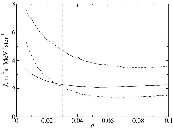
Figure 5. 180 MeV proton intensity at 20 AU (dot-dashed line) and at 95 AU (dashed line) at the V1 latitude and longitude (dashed line), as a function of the ratio κ⊥/κ∥. The solid line is 1 GeV intensity at 20 AU, same latitude/longitude, multiplied by 2.
Download figure:
Standard image High-resolution imagePerpendicular diffusion affects cosmic-ray transport in a number of ways. For example, larger κ⊥ allows the particles access to larger regions of space, e.g., to a broader range of latitudes. The key to understanding the results of Figure 5, however, lies in acceleration at the TS. During A < 0 solar minima ion transport in the SW is not strongly affected by the value of perpendicular diffusion because the principal mode of transport is drift along the neutral sheet. However, larger perpendicular diffusion means particles spend less time in the heliosheath and near the TS, where they are re-accelerated. Evidently, when κ⊥ is small, particles stay close to the shock for extended periods of time and gain more energy, whereas when κ⊥ is large there is virtually no shock acceleration. In performing a simulation where the ∇ · u term was artificially turned off at the TS, we obtained an essentially flat dependence of intensities on a, which confirms our conjecture of the role of the TS. It should be noted, however, that the result reported here may be a consequence of using a flat neutral sheet in the SW. A simulation with a tilted neutral sheet will be required to generalize this result to realistic solar minimum conditions.
All three curves in Figure 5 exhibit a slight upturn at the high end of the range of a considered. Although we do not expect a to exceed 0.1 in the real heliosphere (Zank et al. 2004, 2006), we verified that very large a ∼ 0.5 yielded higher intensities. If diffusion coefficients were this large, ions would spend very little time inside the heliosphere (both in the SW and the heliosheath) and would consequently experience less overall modulation.
5. DISCUSSION
The stochastic Parker model introduced here is an alternative to the more conventional grid-based energetic particle transport models. Its main advantages lie in simplicity and simulation speed. The latter allows to quickly explore the parameter space of the problem, something that would normally take many CPU-months with a four-dimensional global grid code. Another advantage of the stochastic model is the availability of trajectories. This allows to calculate and compare particle residence times in different regions of the heliosphere.
Sample particle trajectories serve to illustrate the physics of transport in the various parts of the heliosphere. Figure 6 shows the ecliptic-plane projections of two representative stochastic trajectories of GCR protons with final energies 100 MeV and 1 GeV (all results were produced with the LZP version of κ⊥). Also shown in this figure are the locations of the heliospheric boundaries. Here, we make the distinction between the heliosheath and heliotail. To our knowledge, there is no accepted definition of the boundary between the two. Here, we define this boundary as the plane perpendicular to the interstellar flow direction 200 AU downstream from the Sun.

Figure 6. Two sample stochastic trajectories starting (in the sense of time-backward simulations) at 30 AU in the ecliptic plane. Shown are projections of the trajectories onto the ecliptic plane. The blue line is the trajectory of a particle with final energy 100 MeV and the red line is the trajectory with final energy 1 GeV. The exit points on the HP are marked with color circles. The shapes of the TS and the HP (also in the ecliptic) are shown and the three different regions (SW, heliosheath, and heliotail) are labeled.
Download figure:
Standard image High-resolution imageBoth trajectories shown start at 30 AU in the ecliptic plane, in the nose direction. Because these are time-backward simulations, starting points can be though of as locations of cosmic-ray "detectors." Each trajectory segment corresponds to a distance traveled in 2 hr time. It is seen that each trajectory executes broad longitudinal sweeps along the direction of B. SW advection adds a gradual radial scan, while drifts and perpendicular diffusion make particles switch to different field lines resulting in a more rapid radial motion. The 100 MeV (blue) particle entered the heliosphere in the tail with a starting energy of 378 MeV. It has spent 460 days in the SW region and 330 days in the heliosheath and heliotail. Because of its long residence time in the SW the blue particle has lost most of its initial energy. The 1 GeV (red) proton entered near the nose having an energy of 1.1 GeV. Its residence time was 100 and 220 days in the SW and the heliosheath–heliotail, respectively. Evidently, any individual cosmic ray observed in the inner heliosphere has, prior to its absorption by the detector, sampled vast volumes of the surrounding space of the outer heliosphere. Including transport in these outlying regions is a necessity for a GCR model to be a valid approximation to physical reality.
Figure 7 shows the mean lengths of time that the stochastic trajectories spend in each of the three regions of the heliosphere as a function of the final proton energy. The left panel is for particles observed at 20 AU, and the right panel is for particles observed at 95 AU, both for the current latitude of V2 (55° in our coordinate system). The lengths of each stack bar is the average time, in days, that particles with each final energy spend in the SW (red), the heliosheath (green), and the heliotail (blue). Each stack bar was produced by averaging residence times over 10,000 stochastic trajectories.

Figure 7. Residence times in the three regions of the heliosphere (in days) vs. kinetic energy for particles observed at (a) r = 20 AU, θ = 55°, ϕ = 0, and (b) r = 95 AU, θ = 55°, ϕ = 0, using the LZP diffusion model. The lengths of the stacked bars correspond to, from the lowest to the highest, residence times in the SW, in the heliosheath, excluding the heliotail, and in the heliotail only.
Download figure:
Standard image High-resolution image
As expected, residence times decrease with increasing energy. At 100 MeV residence times in the heliosheath and tail are ∼3 times longer than in the supersonic SW, with total heliospheric residence time of the order of three years. With increasing energy SW residence times decrease faster than heliosheath residence times, and at the high end of the energy range particles spend ∼6 times as long in the sheath + tail as they do in the SW. Interestingly, residence times of particles observed at 95 AU are often larger than those observed at 20 AU at the same final energy. The trend is particularly strong at low energies. Here, not only the heliosheath, but also SW residence times are larger at 95 AU. The reason for this is that low-energy ions have lower probabilities to reach 95 AU directly from the CHISM than GeV ions (particles are deflected by the modulation wall and never reach the TS). Evidently, the preferred mode of transport for 100 MeV ions is through momentum space, by starting off as higher-energy ions penetrating into the SW region, where they would cool down and subsequently diffuse back into the heliosheath. We should point out that the residence times calculated here will be different for other parts of the solar cycle and/or for different models of cross-field diffusion.
As pointed out by Ball et al. (2005) the heliosheath region is not efficient in cooling or accelerating particles, compared with the SW and the TS. Nevertheless, the heliosheath's overall effect on modulation is prominent. As mentioned above, the modulation wall deflects a fraction of low-energy ions that never reach the inner heliosphere. At the same time our results show that GCR attenuation is not confined to the region right next to the HP. Instead of a steepening gradient, the Voyagers are expected to see a much more modest, slowly increasing gradient all the way to the HP. The modulation wall is apparently not as efficient a barrier during qA < 0 solar minima. As other times, such as during solar maxima, however, its modulation role could be more dominant (Webber & Lockwood 2004).
Results reported here suggest that the TS is not a very efficient accelerator of GCRs. In contrast to Florinski et al. (2003), Ball et al. (2005), and Ferreira & Scherer (2006), our calculated GCR intensities at the shock were never in excess of their interstellar values. Such an excess would appear to be incompatible with both the recent Voyager results and the CHISM spectrum prediction of Webber & Higbie (2009). It should be kept in mind, however, that the solar minimum conditions have not yet been established in the outer heliosphere at the time of writing, and the Voyager intensities could increase further during the next 1–2 years.
We used a two-parameter constraint on our model, namely, the inner heliospheric and the 95 AU spectra. Our results at 95 AU are in agreement with the observations, and the spectra at the inner boundary (10 AU in this work) are generally consistent with observations at the Earth. During the solar minimum particle transport is not very sensitive to the details of the mean free paths or the ratio κ⊥/κ∥. Perpendicular diffusion will affect latitudinal gradients, which could provide additional parameter constraints.
The present model has many venues for improvement. The assumption of a flat neutral sheet in the SW is only approximate—the smallest measured tilt angles are of the order of 5%–10% (http://wso.stanford.edu). A more realistic solar-minimum model must take the tilt angle into account. It would be desirable to extend the MHD model down to 1 AU to permit a direct comparison with observations at the Earth and Ulysses. Conversely, the external boundary, at 1000 AU, has negligible effects on the results because less than 1% of all simulated trajectories leave the simulation domain through the tail. This means there is no need to include the distant heliotail in a simulation unless studying fluxes very far downstream from the Sun. The heliospheric turbulence model used here is somewhat crude and a more refined approached based on the Bartol model (Breech et al. 2008) will be developed in the future.
Our present model does not resolve the north–south asymmetry of the heliosphere reported by the Voyagers (Richardson et al. 2008a; Stone et al. 2008). This asymmetry is difficult to reproduce in a model that includes neutral hydrogen atoms (Pogorelov et al. 2007). By carefully choosing the strength and direction of the CHISM magnetic field it should be possible to identify a configuration that offers the best fit to the Voyager results (Opher et al. 2006; Pogorelov et al. 2007; Izmodenov 2009). Another venue for improvement would be adding a more accurate description of the solar cycle in the heliosheath. A two-dimensional model that included elements of the solar cycle was presented by Ferreira & Scherer (2006). As pointed out by Nerney et al. (1995) several solar cycles may be present in the heliosheath and the heliotail in a compressed form. The resulting magnetic field topology consists of "pockets" of oppositely directed heliomagnetic field and regions filled with a rapidly oscillating neutral sheet. These details will be included in the next generation of three-dimensional MHD-neutral models (Pogorelov et al. 2009).
This research was supported, in part, by NASA grants NNG05GD43G, NNG06GD45G, NNG06GD48G, and NNX08 AJ21G. V.F. thanks F. B. McDonald, A. C. Cummings, G. P. Zank, G. M. Webb, G. Li, and J. Heerikhuisen for helpful discussions. The authors thank M. Potgieter for reviewing the manuscript.