


ABSTRACT
We compare the ∼1 MHz type III bursts of flares associated with samples of "impulsive" and "gradual" solar energetic particle (SEP) events from cycle 23. While large gradual SEP events had much higher > 30 MeV proton intensities, the median-integrated intensities, peak intensities, and durations of the two groups of radio bursts were comparable. Thus, the median "proton yield" (peak > 30 MeV proton intensity of an SEP event divided by its associated integrated ∼1 MHz intensity) of type III bursts associated with gradual SEP events was ∼280 times larger than that for impulsive SEP events. A similar yield difference of ∼250 was observed for 4.4 MeV electron events. Only for extrapolated electron energies ∼5 keV, corresponding to the energy of the electrons that excite type III emission, does the median yield converge to the same value for both groups of events. The time profiles of ∼1 MHz bursts associated with impulsive SEP events are characteristically shorter and simpler than those associated with the gradual SEP events, reflecting the development of the second stage of radio emission in large eruptive flares. The gradual SEP events were highly associated (96%) with decametric-hectometric (DH) type II bursts versus only a 5% association rate for the impulsive events. Large favorably located ∼1 MHz type III bursts with associated DH type IIs had an ∼60% association rate with large (≥ 1 pfu) > 30 MeV SEP events versus ∼5% for ∼1 MHz bursts without accompanying DH II emission. These results are interpreted in terms of two distinct types of particle acceleration at the Sun, a flare-resident process that produces relatively few > 30 MeV protons and ∼4 MeV electrons in space and a shock process that dominates the large gradual proton events.
Export citation and abstract BibTeX RIS
1. INTRODUCTION
Low-frequency radio bursts have long indicated that the Sun has two primary particle acceleration mechanisms: an impulsive flare-resident reconnection-based process, for which fast-drift type III (drift rate ∼100 MHz s−1 in the metric range) bursts are the characteristic emission, and a delayed process characterized by slow-drift (∼0.1–1 MHz s−1) type II emission, attributed to a shock moving out in the solar corona with a speed of ∼1000 km s−1 (Wild 1985). These emissions, attributed to streams of electrons and magnetohydrodynamic shock waves, respectively, are shown in the schematic spectrogram of a fully-developed radio event in Figure 1. Much more commonly, only the first phase, characterized by type III bursts and corresponding to the first ∼5 minutes in Figure 1, is observed.
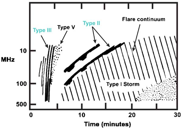
Figure 1. Schematic diagram of a fully-developed solar radio burst (adapted from Dulk et al. 1985).
Download figure:
Standard image High-resolution imageWild et al. (1963) proposed that it is the second phase shock process that is responsible for acceleration of solar protons and relativistic electrons, a view that gained general acceptance as evidence on particle event composition and charge states accumulated during the space age (Reames 1993, 1999). In this picture, small first-phase (impulsive) events are deficient in protons, rich in 3He and Fe, and exhibit high charge states of Fe, suggestive of a flare process, while large (gradual) solar energetic particle (SEP) events are proton-rich, 3He- and Fe-poor, and have low Fe charge states characteristic of the ambient corona.
Recently, the two-class picture had been challenged by new observations. Composition and charge state measurements (Cohen et al. 1999a, 1999b; Mazur et al. 1999; Labrador et al. 2001; also see Mewaldt et al. 2006) at > 10 MeV amu−1 revealed that certain large, and therefore presumably gradual, i.e., shock-dominated, SEP events had flare-like composition (1997 November 6, 1998 May 2, 1998 May 6, 1998 November 14) and charge state (1997 November 6, 1998 November 14) characteristics. This development prompted suggestions (e.g., Cliver 2000a, 2000b; Cane et al. 2003) that the flare process was making a more significant contribution in these large events than had been previously thought to be the case. Cane et al. (2002) linked ∼20 MeV proton events to extended complex type III bursts most easily observed at low frequencies (< 14 MHz) from space. They reported: "For the majority of the particle events, in particular those [larger events] that lasted longer than 36 hr, the type III activity is not just an extension of "normal" type III bursts that occur in the initial, impulsive, phase of flare events but, rather it continues or starts some 5–10 minutes later. The type III emission [termed "type III-l"] lasts on average about 20 minutes at 14 MHz as compared with "normal" type III groups at flare onset that last about 5 minutes." Cane et al. (2003) suggested that the flare process, as manifested by type III-l bursts, dominated ion acceleration at energies > 25 MeV amu−1. A subsequent study by Cane et al. (2006) made the more modest suggestion that a delayed flare-resident (i.e., type III-l associated) acceleration process could contribute to large SEP events.
What are the relative contributions of the flare-resident (type III) and shock (type II) acceleration processes in large > 25 MeV amu−1 SEP events? In this study, we address this question by examining the properties of low-frequency (∼1 MHz) type III bursts observed by Wind/Waves (Bougeret et al. 1995) for two groups of bursts. The first set of ∼1 MHz bursts is associated with a sample of large impulsive SEP events from cycle 23 identified by Reames & Ng (2004) on the basis of their high-Z (Fe and above) elemental abundances. The second group consists of a sample of large gradual SEP events recorded during this same period. Following Cane et al. (2002), the impulsive SEP events are linked to "normal" type IIIs and the large gradual events are identified with "type III-l" bursts.
If, as argued by Cane et al. (2003), > 25 MeV protons accelerated in the flare-resident acceleration process play a major role in large SEP events, we would expect the size of the proton events to scale with the energy of the associated type III bursts—the characteristic radio emission of the SEP acceleration process in flares. Specifically, we would expect the normal type IIIs associated with impulsive SEP events to be less energetic, i.e., to have smaller time-integrated radio fluxes, than the type III-ls associated with the sample of large gradual events. This hypothesis is based on (i) the report by Cane et al. (2002) that "SEP events become more intense as the type III activity becomes longer lasting" and (ii) the earlier finding by Cane et al. (1981) that "SA [shock-accelerated] events [as type III-ls were originally called] are generally more intense than [normal] type III bursts." To test this supposition, we examine the "proton yields" (proton intensity divided by time-integrated type III intensity) of the two groups by normalizing them for the sizes of the associated type III bursts. Assuming that "the causative electrons [in type III-ls] are ... accelerated in the same manner as for normal type III bursts (Cane et al., 2002)," we would expect the > 25 MeV proton yields to be the same for the two groups of events. If they are not, it would imply either that the flare-resident process changes in character as it is prolonged in time or that the underlying assumption that > 25 MeV proton acceleration is dominated by the flare process is incorrect.
To gain further insight into the relative contributions of flares and shocks to large SEP events, we compare the durations and complexity of the associated ∼1 MHz type III bursts for both of our SEP samples and determine the association of the two groups with decametric-hectometric (DH) type II bursts. Finally, we conduct a reverse study beginning with a comprehensive list of large favorably-located ∼1 MHz type III bursts from 1997 to 2004 and determine the effect of DH type II bursts on their associations with large > 30 MeV proton events.
Our analysis is presented in Section 2 and the results are summarized and discussed in Section 3.
2. DATA ANALYSIS
2.1. Data Tables
2.1.1. Event Selection
Our sample of "impulsive" events was taken from Table 1 of Cliver & Ling (2007). It consists of the large impulsive events identified by Reames & Ng (2004) for which Nitta et al. (2006) identified associated flares between W20 and W89, where the longitude restriction is applied to reduce particle propagation and radio burst occultation effects. Reames & Ng selected their impulsive events by scanning hourly-averaged data from 1994 November to 2003 September for events with Fe/O >0.5 (not normalized to coronal values, for 3.3–10 MeV amu−1) and peak Fe intensities greater than 10−4 particles cm−2 sr−1 s−1 MeV−1 amu−1 at 2.4–3.2 MeV amu−1. Our list of large (J (>10 MeV) ≥ 10 proton flux units (pfu) in hourly-averaged data; 1 pfu = 1 pr cm−2 s−1 sr−1) "gradual" well-connected (W20–W89) proton events was taken from Table 1 of Cane et al. (2006).3 As a final restriction on both lists of events, we only considered events for which Wind/Wave observations were available on line at 940 MHz (this eliminated, roughly, 2003 August–November and all of 2005; we did not consider 2006–present). Our samples of 22 impulsive and 25 gradual events are given in Tables 1 and 2, respectively.
Table 1. Large Impulsive SEP Events
| GOES SXR | Wind/Waves Type III | SEPsa | |||||||||||||
|---|---|---|---|---|---|---|---|---|---|---|---|---|---|---|---|
| Date and Time | Class | Location | Start Time | Duration | Int. Intensity | Profile | DH Type II | GOES >30 MeV pr flux | GOES >10 MeV pr flux | SOHO 4.4 MeV e-flux | SOHO 1.8 MeV e-flux | SOHO 0.5 MeV e-flux | ACE 50 keV e-flux | >30 MeV Proton Yield | |
| 1 | 1997 Sep 18 00:01 | C 1.6 | S25W76 | 23:59 | 6 | 1.87 × 10⁵ | S | ... | 8.91 × 10⁻²(A) | 1.30 × 10⁻¹(A) | 2.49 × 10⁻³(U) | 3.13 × 10⁻² | 2.18 × 101 | 9.92 × 10³ | 4.76 × 10⁻⁷ |
| 2 | 1998 Sep 27 08:13 | C 2.8 | N21W48 | 08:09 | 17 | 1.32 × 10⁷ | S | ... | 2.72 × 10⁻² | 2.35 × 10⁻¹ | G | G | 1.78 × 10⁴(A) | 1.79 × 10⁵ | 2.06 × 10⁻⁹ |
| 3 | 1998 Sep 27 23:42 | C 6.5 | N20W58 | 23:39 | 14 | 5.59 × 10⁶ | S | ... | 7.69 × 10⁻²(U) | 4.01 × 10⁻² | G | G | 6.88 × 10³(A) | 9.03 × 10⁴ | 1.38 × 10⁻⁸ |
| 4 | 1998 Sep 29 02:02 | C 6.6 | N23W69 | 01:58 | 12 | 6.58 × 10⁶ | S | ... | 8.41 × 10⁻²(U) | 3.00 × 10⁻² | G | G | 8.09 × 10²(A) | 3.60 × 10⁴ | 1.28 × 10⁻⁸ |
| 5 | 1999 Feb 20 04:06 | C 8.7 | S18W63 | 03:58 | 24 | 4.37 × 10⁶ | N | ... | 2.56 × 10⁻²(A) | 3.55 × 10⁻²(A) | 6.35 × 10⁻⁴ | 4.06 × 10⁻² | 1.69 × 101 | 1.03 × 10⁴ | 5.86 × 10⁻⁹ |
| 6 | 1999 Feb 20 15:19 | C 4.4 | S21W72 | 15:14 | 23 | 5.95 × 10⁶ | C | ... | 9.84 × 10⁻²(U) | 1.67 × 10⁻¹(U) | 2.88 × 10⁻³(U) | 3.24 × 10⁻² | 1.61 × 101 | 3.59 × 10³ | 1.65 × 10⁻⁸ |
| 7 | 1999 Aug 7 17:04 | C 2.2 | N22W74 | 17:04 | 7 | 8.66 × 10⁵ | S | ... | 9.78 × 10⁻²(U) | 1.64 × 10⁻¹(U) | 3.89 × 10⁻³(U) | 1.16 × 10⁻² | 5.84 × 100 | 3.22 × 10³ | 1.13 × 10⁻⁷ |
| 8 | 1999 Dec 27 01:54 | M 1.1 | N24W35 | 01:50 | 16 | 3.86 × 10⁶ | C | ... | 9.65 × 10⁻³(A) | 2.54 × 10⁻²(A) | 1.35 × 10⁻³ | 6.73 × 10⁻¹ | 2.34 × 10² | 1.02 × 10⁴ | 2.50 × 10⁻⁹ |
| 9 | 2000 Mar 7 12:33 | C 3.9 | S15W72 | 12:31 | 10 | 1.68 × 10⁵ | S | ... | 7.49 × 10⁻³(A) | 1.99 × 10⁻²(A) | 2.63 × 10⁻³(U) | 1.82 × 10⁻¹ | 1.15 × 10² | 9.78 × 10³ | 4.45 × 10⁻⁸ |
| 10 | 2000 Mar 7 23:40 | C 5.0 | S15W76 | 23:40 | 11 | 1.14 × 10⁶ | S | ... | 3.00 × 10⁻² | 2.69 × 10⁻² | 2.88 × 10⁻³(U) | 1.13 × 10⁻¹ | 7.75 × 101 | 1.77 × 10³ | 2.64 × 10⁻⁸ |
| 11 | 2000 May 1 10:26 | M 1.2 | N21W50 | 10:19 | 12 | 4.50 × 10⁵ | S | ... | 8.23 × 10⁻² | 1.85 × 10⁻¹ | 1.24 × 10⁻² | 6.03 × 100 | 3.55 × 10³ | 1.56 × 10⁵ | 1.83 × 10⁻⁷ |
| 12 | 2000 May 23 20:53 | M 1.0 | N21W42 | 20:42 | 25 | 7.48 × 10⁶ | C | ... | 1.91 × 10⁻²(A) | 8.48 × 10⁻² | 6.48 × 10⁻³ | 8.04 × 10⁻¹ | 3.36 × 10² | 5.25 × 10⁴ | 2.55 × 10⁻⁹ |
| 13 | 2000 Jun 4 07:09 | C 1.1 | S10W62 | 07:03 | 10 | 3.22 × 10⁶ | S | ... | 1.37 × 10⁻²(A) | 1.42 × 10⁻²(A) | 6.94 × 10⁻⁴ | 6.19 × 10⁻² | 2.82 × 101 | 2.20 × 10⁴ | 4.27 × 10⁻⁹ |
| 14 | 2000 Aug 12 12:40 | C 2.5 | N05W48 | 12:31 | 4 | 1.84 × 10⁴ | N | ... | 3.94 × 10⁻² | 4.77 × 10⁻¹ | 1.18 × 10⁻³ | 1.24 × 100 | 6.15 × 10² | 2.69 × 10⁵ | 2.14 × 10⁻⁶ |
| 15 | 2001 Apr 14 17:22 | C 4.5 | S18W71 | 17:10 | 69 | 1.49 × 10⁷ | C | ... | 6.67 × 10⁻² | 4.60 × 10⁻¹ | 9.24 × 10⁻³ | 5.64 × 100 | 3.64 × 10³ | 2.71 × 10⁵ | 4.49 × 10⁻⁹ |
| 16 | 2002 Apr 14 22:29 | C 7.6 | N18W75 | 22:26 | 14 | 4.02 × 10⁶ | N | ... | 1.91 × 10⁻² | 1.20 × 10⁻¹ | 6.33 × 10⁻⁴ | 1.50 × 10⁻¹ | 7.84 × 101 | 8.76 × 10³ | 4.75 × 10⁻⁹ |
| 17 | 2002 Apr 15 02:51 | M 1.1 | N20W79 | 02:46 | 17 | 2.53 × 10⁶ | N | ... | 2.15 × 10⁻² | 9.19 × 10⁻² | 1.24 × 10⁻³ | 5.53 × 10⁻¹ | 2.71 × 10² | 1.96 × 10⁴ | 8.51 × 10⁻⁹ |
| 18 | 2002 Aug 3 19:07 | X 1.2 | S16W80 | 18:59 | 23 | 1.78 × 10⁶ | N | Y | 5.38 × 10⁻² | 1.88 × 10⁻¹ | 4.75 × 10⁻³ | 7.76 × 10⁻¹ | 2.85 × 10² | 2.16 × 10⁴ | 3.03 × 10⁻⁸ |
| 19 | 2002 Aug 18 21:24 | M 2.2 | S13W20 | 21:13 | 25 | 8.88 × 10⁶ | C | ... | 3.12 × 10⁻¹ | 2.59 × 100 | 1.29 × 10⁻² | 3.84 × 100 | 1.91 × 10³ | 9.49 × 10⁴ | 3.52 × 10⁻⁸ |
| 20 | 2002 Aug 19 10:34 | M 2.2 | S12W26 | 10:30 | 18 | 7.63 × 10⁶ | S | ... | 6.70 × 10⁻² | 7.58 × 10⁻¹ | 4.06 × 10⁻² | 8.28 × 100 | 8.57 × 10³ | 3.75 × 10⁵ | 8.78 × 10⁻⁹ |
| 21 | 2002 Aug 19 21:02 | M 3.4 | S11W32 | 20:57 | 18 | 2.63 × 10⁶ | N | ... | 3.30 × 10⁻² | 1.68 × 10⁻¹ | 6.64 × 10⁻³ | 5.88 × 100 | 3.44 × 10³ | 8.73 × 10⁴ | 1.25 × 10⁻⁸ |
| 22 | 2002 Aug 20 08:26 | M 3.5 | S11W38 | 08:25 | 15 | 1.04 × 10⁷ | S | ... | 2.71 × 10⁻¹ | 1.47 × 100 | 4.26 × 10⁻¹ | 9.51 × 101 | 4.29 × 10⁴ | 2.63 × 10⁵ | 2.61 × 10⁻⁸ |
Notes. aProton Flux Units = protons cm−2 s−1 sr−1; Electron Flux Units = electrons cm−2 s−1 sr−1 MeV−1; Yield Units = pfu sfu−1 minute−1; (A) = intensity derived from ACE measurement; (U) = upper limit; G = data gap. For SEP events for which the peak intensity was less than 10 times the pre-event background, we subtracted the pre-event intensity. For all SEP channels, peak intensities were taken within ∼12 hr of the SXR maximum (see Cliver & Ling 2007). For event Nos. 8, 11, and 21, the ∼1 MHz background was greater than 2000 sfu at the time of burst onset; for these cases, we used the visually determined burst onset time.
Download table as: ASCIITypeset image
Table 2. Gradual SEP Events
| GOES SXR | Wind/Waves Type III | SEPsa | |||||||||||||
|---|---|---|---|---|---|---|---|---|---|---|---|---|---|---|---|
| Date and Time | Class | Location | Start Time | Duration | Int. Intensity | Profile | DH Type II | GOES > 30 MeV pr Flux | GOES >10 MeV pr Flux | SOHO 4.4 MeV e-Flux | SOHO 1.8 MeV e-Flux | SOHO 0.5 MeV e-Flux | ACE 50 keV e-Flux | >30 MeV Proton Yield | |
| 1 | 1997 Nov 4 05:58 | X 2.1 | S14W33 | 05:57 | 30 | 1.73 × 10⁷ | N | Y | 1.69 × 101 | 5.48 × 101 | 2.08 × 100 | 4.70 × 101 | 1.45 × 10⁴ | 1.94 × 10⁵ | 9.74 × 10⁻⁷ |
| 2 | 1997 Nov 6 11:55 | X 9.4 | S18W63 | 11:53 | 35 | 2.50 × 10⁷ | N | Y | 1.79 × 10² | 4.39 × 10² | 3.24 × 101 | 4.99 × 10² | 1.18 × 10⁵ | 7.64 × 10⁵ | 7.14 × 10⁻⁶ |
| 3 | 1998 May 6 08:09 | X 2.8 | S11W65 | 07:59 | 44 | 1.03 × 10⁷ | C | Y | 3.83 × 101 | 1.42 × 10² | 1.75 × 101 | 3.24 × 10² | 1.03 × 10⁵ | 1.27 × 10⁶ | 3.71 × 10⁻⁶ |
| 4 | 1998 Sep 30 13:48 | M 3.0 | N19W85 | 13:27 | 36 | 7.45 × 10⁵ | C | Y | 1.12 × 10² | 9.79 × 10² | G | G | 2.31 × 10⁵(A) | 7.70 × 10⁵ | 1.50 × 10⁻⁴ |
| 5 | 1999 Jun 4 07:03 | M 4.2 | N17W69 | 06:51 | 33 | 3.94 × 10⁶ | C | Y | 2.80 × 100 | 5.08 × 101 | 2.15 × 10⁻¹ | 4.31 × 101 | 1.07 × 10⁴ | 1.43 × 10⁵ | 7.10 × 10⁻⁷ |
| 6 | 2000 Apr 4 15:39 | M 1.0 | N16W66 | 15:17 | 26 | 9.47 × 10⁶ | C | Y | 6.52 × 10⁻¹ | 3.17 × 101 | 8.93 × 10⁻³ | 3.43 × 100 | 1.16 × 10³ | 8.25 × 10⁴ | 6.88 × 10⁻⁸ |
| 7 | 2000 Jun 10 17:00 | M 5.6 | N22W40 | 16:54 | 35 | 1.93 × 10⁷ | C | Y | 1.02 × 101 | 4.07 × 101 | 5.02 × 10⁻¹ | 2.96 × 101 | 5.40 × 10³ | 1.74 × 10⁵ | 5.30 × 10⁻⁷ |
| 8 | 2000 Jul 22 11:32 | M 3.9 | N14W56 | 11:33 | 13 | 1.41 × 10⁵ | S | Y | 3.36 × 100 | 1.38 × 101 | 4.45 × 10⁻² | 7.73 × 100 | 1.70 × 10³ | 2.78 × 10⁴ | 2.39 × 10⁻⁵ |
| 9 | 2000 Nov 8 23:27 | M 7.9 | N10W75 | 22:55 | 26 | 5.48 × 10⁶ | C | Y | 4.22 × 10³ | 1.15 × 10⁴ | 8.72 × 10² | 4.17 × 10³ | 5.44 × 10⁵ | 3.39 × 10⁶ | 7.69 × 10⁻⁴ |
| 10 | 2001 Jan 28 15:58 | M 1.7 | S04W59 | 15:44 | 31 | 1.64 × 10⁶ | C | Y | 4.71 × 100 | 2.78 × 101 | 1.24 × 10⁻¹ | 1.81 × 101 | 4.46 × 10³ | 5.80 × 10⁴ | 2.88 × 10⁻⁶ |
| 11 | 2001 Apr 2 21:50 | X18.4 | N17W78 | 21:47 | 35 | 2.91 × 10⁶ | N | Y | 1.45 × 10² | 6.59 × 10² | 2.40 × 101 | 4.12 × 10² | 7.58 × 10⁴ | 7.49 × 10⁵ | 4.97 × 10⁻⁵ |
| 12 | 2001 Apr 12 10:28 | X 2.2 | S20W42 | 10:18 | 33 | 6.58 × 10⁶ | C | Y | 1.20 × 101 | 3.90 × 101 | 7.02 × 10⁻¹ | 1.07 × 101 | 4.86 × 10³ | 4.76 × 10⁴ | 1.83 × 10⁻⁶ |
| 13 | 2001 Apr 15 13:50 | X15.8 | S20W84 | 13:47 | 37 | 1.08 × 10⁷ | C | Y | 5.94 × 10²(A) | 9.00 × 10² | 1.00 × 10² | 8.56 × 10² | 1.38 × 10⁵ | 6.68 × 10⁵ | 5.50 × 10⁻⁵ |
| 14 | 2001 Nov 22 23:27 | X 1.0 | S15W34 | 23:13 | 16 | 1.25 × 10⁵ | C | Y | 5.55 × 10² | 2.99 × 10³ | 7.93 × 101 | 4.92 × 10² | 7.10 × 10⁴ | 5.43 × 10⁵ | 4.44 × 10⁻³ |
| 15 | 2001 Dec 26 05:36 | M 7.6 | N08W54 | 05:12 | 22 | 1.17 × 10⁶ | C | Y | 2.83 × 10² | 7.24 × 10² | 2.86 × 101 | 2.17 × 10² | 6.20 × 10⁴ | 7.28 × 10⁵ | 2.43 × 10⁻⁴ |
| 16 | 2002 Mar 18 02:30 | M 1.1 | S09W46 | 02:20 | 10 | 2.38 × 10⁵ | N | Y | 9.66 × 10⁻¹ | 1.93 × 101 | 6.55 × 10⁻² | 1.10 × 101 | 9.39 × 10³ | 1.94 × 10⁵ | 4.07 × 10⁻⁶ |
| 17 | 2002 Apr 21 01:47 | X 1.7 | S14W84 | 01:21 | 39 | 4.30 × 10⁶ | C | Y | 6.34 × 10² | 2.09 × 10³ | 8.93 × 101 | 7.08 × 10² | 1.49 × 10⁵ | 8.08 × 10⁵ | 1.47 × 10⁻⁴ |
| 18 | 2002 Aug 14 02:11 | M 2.6 | N09W54 | 01:52 | 32 | 9.50 × 10⁵ | C | Y | 3.05 × 10⁻¹ | 1.14 × 101 | 1.27 × 10⁻² | 3.08 × 100 | 4.47 × 10³ | 3.49 × 10⁵ | 3.21 × 10⁻⁷ |
| 19 | 2002 Aug 22 01:57 | M 5.9 | S07W62 | 01:46 | 24 | 1.08 × 10⁷ | N | ... | 1.01 × 101 | 3.13 × 101 | 3.92 × 10⁻¹ | 2.19 × 101 | 4.23 × 10³ | 1.22 × 10⁵ | 9.39 × 10⁻⁷ |
| 20 | 2002 Nov 9 13:23 | M 4.9 | S12W29 | 13:09 | 29 | 8.05 × 10⁶ | C | Y | 8.31 × 100 | 2.14 × 10² | 7.46 × 10⁻¹ | 3.24 × 101 | 1.33 × 10⁴ | 3.40 × 10⁵ | 1.03 × 10⁻⁶ |
| 21 | 2003 May 31 02:24 | X 1.0 | S07W65 | 02:21 | 15 | 8.43 × 10⁶ | N | Y | 4.91 × 100 | 1.58 × 101 | 1.29 × 100 | 7.04 × 101 | 2.96 × 10⁴ | 5.18 × 10⁵ | 5.82 × 10⁻⁷ |
| 22 | 2004 Apr 11 04:19 | M 1.0 | S14W47 | 03:58 | 20 | 3.02 × 10⁶ | C | Y | 1.35 × 100 | 2.21 × 101 | 1.54 × 10⁻¹ | 2.08 × 101 | 3.77 × 10³ | 7.17 × 10⁴ | 4.47 × 10⁻⁷ |
| 23 | 2004 Jul 25 15:15 | M 1.2 | N08W33 | 14:32 | 3 | 3.55 × 10⁴ | N | Y | 2.05 × 100 | 3.83 × 101 | 3.03 × 10⁻¹ | 4.93 × 101 | 8.03 × 10³ | 1.02 × 10⁵ | 5.77 × 10⁻⁵ |
| 24 | 2004 Sep 19 17:11 | M 2.0 | N03W58 | 17:01 | 25 | 4.23 × 10⁶ | C | Y | 7.86 × 100 | 4.58 × 101 | G | G | 7.50 × 10⁴(A) | 1.10 × 10⁵ | 1.86 × 10⁻⁶ |
| 25 | 2004 Nov 10 02:13 | X 2.8 | N09W49 | 02:11 | 26 | 1.95 × 10⁶ | C | Y | 4.05 × 101 | 2.64 × 10² | 4.29 × 100 | 1.07 × 10² | 2.41 × 10⁴ | 1.79 × 10⁵ | 2.08 × 10⁻⁵ |
Notes. aProton Flux Units = protons cm−2 s−1 sr−1; Electron Flux Units = electrons cm−2 s−1 sr−1 MeV−1; Yield Units = pfu sfu−1 minute−1; (A) = intensity derived from ACE measurement; G = data gap. For SEP events for which the peak intensity was less than 10 times the pre-event background, we subtracted the pre-event intensity. For all SEP channels, peak intensities were taken within ∼12 hr of the SXR maximum (see Cliver & Ling 2007). For event Nos. 5 and 7, the ∼1 MHz background was greater than 2000 sfu at the time of burst onset; for these cases, we used the visually determined burst onset time.
Download table as: ASCIITypeset image
2.1.2. Radio Data
One-minute averages of the Wind/Waves data4 were converted from units of dBm to solar flux units (sfu; 1 sfu = 10−22 Watts m−2 Hz−1). To quantify the type III radio emission for the events listed in Tables 1 and 2, we used a frequency of ∼1 MHz (specifically 940 kHz), the closest frequency to 1 MHz at which measurements have been made in the RAD1 receiver for most of the Wind lifetime. For the density model of Leblanc et al. (1998), a frequency of 1 MHz corresponds to an emission height of ∼7 Rs (measured from the Sun center). At this frequency/height, the emission is due to electrons that have escaped from the Sun and have passed beyond any associated coronal mass ejection (CME) and shock that might disrupt the "bump-on-tail" instability required to generate the type III burst (Reiner et al. 2007). For each event in Tables 1 and 2, we made a two-panel plot showing time profiles of the 1–8 Å soft X-ray (SXR) emission observed by the Geostationary Operational Environmental Satellites (GOES) and the ∼1 MHz radio emission observed by Wind/Waves. Examples of two of these plots are given in Figures 2a and 2b, respectively. Using the SXR curve as a guide, as well as specifications of type III intervals for 13 of our gradual events (Table 2) given in Cane et al. (2002), we first visually determined the start and end times of the associated type III radio emission, comparing against the spectrograms given on the Waves Web site. From inspection of these plots, we determined an intensity level—of 2 × 10³ sfu—at which to automatically start and end burst integrations for the largest peak in the visually selected interval, interpolating across short data gaps as necessary. The burst durations, obtained in this manner, were shorter than those determined visually. Because the type III bursts were generally dominated by a single (either simple or complex) peak, however, the integrated intensities were comparable in most cases. Of the 47 events in Tables 1 and 2, the automatically determined integrated ∼1 MHz intensity was within 5% of that with visually determined intervals for 41 cases and within 10% for 44. For the three smallest ∼1 MHz events in the sample, the mechanically determined value was ∼20% lower in one case, a factor of ∼2 lower in another, and a factor of ∼3 lower in the third. As will be seen below, these discrepancies do not affect our conclusions.

Figure 2. (a) 1–8 Å time profile (top) and ∼1 MHz time profile (bottom) for the flare associated with the impulsive SEP event at 08:13 UT on 1998 September 27. (b) 1–8 Å time profile (top) and ∼1 MHz time profile (bottom) for the flare associated with the gradual SEP event on 2004 September 19. The dashed vertical lines mark the peak time of the SXR burst and the cross-hatching in the lower panel indicates the integrated radio intensities used in the analysis.
Download figure:
Standard image High-resolution image2.1.3. Particle Data
The tabulated particle data in Tables 1 and 2 were taken from the following sources. For proton data, we used the GOES spacecraft (GOES-8, -11, -12, and -10; in order of preference, assuming normal operation).5 To check/augment these data, we used > 10 MeV and > 30 MeV proton data from the Solar Isotope Spectrometer (SIS; Stone et al. 1998) on the Advanced Composition Explorer (ACE).6 For electron data, we used the 45 keV (38–53 keV) channel on the ACE Electron, Proton, and Alpha Monitor (EPAM; Gold et al. 1998) and the 0.475 MeV (250–700 keV), 1.835 MeV (0.67–3.0 MeV), and 4.41 MeV (2.64–6.18 MeV) channels from the Comprehensive Suprathermal and Energetic Particle Analyzer (COSTEP; Müller-Mellin et al. 1995) on the Solar and Heliospheric Observatory (SOHO). For periods when COSTEP data were unavailable, such as the COSTEP extended SOHO outage during the second half of 1998, we used a correlation between COSTEP 0.475 MeV electron peak intensities and 175–315 keV electron peak intensities from EPAM to calculate an equivalent intensity (see Cliver & Ling 2007).7 Following Cliver & Ling (2007), our procedure was to select the largest peak (or highest intensity) occurring within ∼12 hr of the 1–8 Å peak of the associated flare, thus restricting our focus to the prompt component of SEP events. For several impulsive events, only upper limits (designated by a (U) in Table 1) were available for proton and/or high-energy electron channels; in our histogram analysis, in Section 2.2, we treated these upper limits as if they were actual values.
2.2. Comparison of Particle and Radio Parameters and "Proton Yields" for Impulsive and Gradual SEP Events
Histograms of the peak > 10 and > 30 MeV proton intensities for the two groups of events are given in Figure 3. The median > 10 MeV (>30 MeV) proton intensity of the sample of large gradual events is a factor of ∼345 (∼220) larger than that of the large impulsive events.

Figure 3. Histograms of the peak > 10 MeV (top) and > 30 MeV (bottom) proton intensities for the impulsive and gradual SEP events analyzed. The medians of the various distributions are marked by arrows.
Download figure:
Standard image High-resolution imageHistograms of the durations, peak intensities, and integrated intensities for the ∼1 MHz emissions for the two groups of events in Tables 1 and 2 are given in Figures 4a–4c, respectively. The differences in the median values of these parameters are much smaller than was the case for the proton intensities. For each of these parameters, the median values of the two groups are within a factor of 2 of each other; gradual events were 1.87 times longer (median duration = 29 minutes versus 15.5 minutes for impulsive events), impulsive events were more intense (median peak flux density = 1.07 × 10⁶ sfu versus 7.87 × 10⁵ sfu) and gradual events had larger integrated flux densities (median value of 4.23 × 10⁶ sfu-minute versus 3.94 × 10⁶ sfu-minute). The longer durations of the ∼1 MHz bursts associated with the large gradual SEP events are somewhat offset by the greater intensities of those associated with the large impulsive events and, as a result, the median-integrated intensities of the two groups are remarkably similar, given their more than 2 orders of magnitude difference in median SEP intensities.
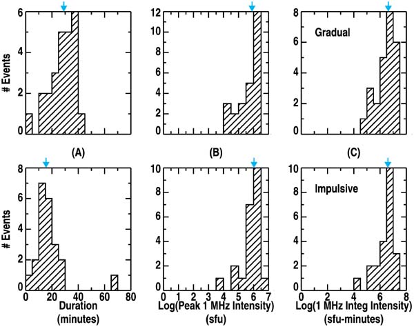
Figure 4. Histograms of the durations (a), peak intensities (b), and integrated intensities (c) for the ∼1 MHz bursts associated with the gradual (top) and impulsive (bottom) SEP events in Tables 1 and 2. The medians of the various distributions are marked by arrows.
Download figure:
Standard image High-resolution imageFigure 5 gives histograms of the "proton yields" at > 10 MeV and > 30 MeV for the impulsive and gradual proton events, respectively, where proton yield is defined as the peak > 10 (or >30) MeV intensity divided by the integrated ∼1 MHz intensity. The median proton yield of the radio bursts associated with the large impulsive > 10 MeV (>30 MeV) proton events is a factor of ∼520 (3.37 × 10⁻⁸ pfu sfu−1 minute−1 versus 1.75 × 10⁻⁵ pfu sfu−1 minute−1) [∼280 (1.32 × 10⁻⁸ pfu sfu−1 minute−1 versus 3.71 × 10⁻⁶ pfu sfu−1 minute−1)] smaller than that of the ∼1 MHz bursts associated with the sample of gradual SEP events. The scatter plot of peak > 30 MeV proton intensity versus integrated ∼1 MHz type III intensity for the two groups of events in Figure 6 shows that our expectation for the size of proton events to scale with the energy of the associated type III bursts does not hold up for the two groups of events. Based on the work of Cane et al. (1981, 2002), we had anticipated that the points corresponding to the impulsive events would have been mainly located in the lower left-hand corner of the plot with the gradual events clustering in the upper right. In this plot, we have flagged (with red circles) two of the large gradual SEP events with impulsive SEP characteristics (Nos. 2 (Fe/O (at 30–40 MeV) = 5.8, normalized to coronal values) and 3 (Fe/O = 4.0) in Table 2; Fe/O values from Tylka et al. 2005) that provoked the current controversy (Cohen et al. 1999a, 1999b) and four additional events (encompassed by red squares) with Fe/O ratios ≥ 4.0 (Nos. 7 (Fe/O = 4.6), 13 (4.8), 15 (4.2), and 19 (4.6) in Table 2). The >30 MeV proton yields for these six events ranged from 5.3 × 10⁻⁷ pfu sfu−1 minute−1 to 2.4 × 10⁻⁴ pfu sfu−1 minute−1, with a median ∼5.4 × 10⁻⁶ pfu sfu−1 minute−1, comparable to that (3.7 × 10⁻⁶ pfu sfu−1 minute−1) of the overall sample for the gradual events and well above that of the impulsive events (1.3 × 10⁻⁸ pfu sfu−1 minute−1).
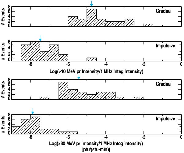
Figure 5. Histograms of the "proton yields" at > 10 MeV (top) and > 30 MeV (bottom) for the impulsive and gradual proton events in our sample. Median yields are marked by arrows.
Download figure:
Standard image High-resolution image
Figure 6. Scatter plot of peak > 30 MeV proton intensity vs. integrated ∼1 MHz type III intensity for the gradual (black filled circles) and impulsive (blue filled circles) SEP events in Tables 1 and 2. Median intensities of the two SEP distributions are indicated by dashed horizontal lines. Two of the large gradual SEP events with impulsive SEP characteristics (Nos. 2 and 3 in Table 2) that provoked the current controversy (Cohen et al. 1999a, 1999b) are indicated by red circles; four additional events (Nos. 7, 13, 15, and 19 in Table 2) with high Fe/O ratios at 30 MeV–40 MeV are indicated by red squares.
Download figure:
Standard image High-resolution imageIn Figure 6, the gap between impulsive and gradual proton intensities is artificial, reflecting our selection of the largest gradual events for comparison with the largest impulsive events, considering that all proton peak intensities will fill up the gap. The figure illustrates that for a given integrated ∼1 MHz intensity, the acceleration process for > 30 MeV protons in large (≥10 pfu for E >10 MeV) gradual SEP events is far more productive than that operating in the largest "pure" impulsive events.
Figures 7a–7d give histograms of electron intensity at 4.41 MeV, 1.835 MeV, 0.475 MeV, and 45 keV, respectively, for the two groups of events. It can be seen that as one goes to lower energies, the two distributions exhibit increasing overlap. In Figures 8a–8d, we show histograms of "electron yields" at 4.41 MeV, 1.835 MeV, 0.475 MeV, and 45 keV, respectively, for the two groups of events (where "electron yield" is defined as for the proton events). As one goes to lower electron energies, the two distributions begin to merge, with the gradual event yields being ∼250 times larger at 4.4 MeV and ∼5 times larger at 50 keV. In Figure 9, we have plotted the difference between the median electron yields for both groups as a function of electron energy. Extrapolating the straight line fit through the four data points indicates that the gradual and impulsive yield distributions merge at an energy ∼5 keV, consistent with the median ∼6 keV energy of exciter electrons deduced for the leading edges of Wind/Waves type III bursts (Haggerty & Roelof 2006; see Kahler & Ragot 2006) and the 2–12 keV energies of electrons that produce Langmuir emission at 1 AU (Ergun et al. 1998). Our interpretation of this result is that a given number of electrons, accelerated by either a flare or shock process, will give the same amount of radio emission. Extrapolation of individual electron spectra (using the 50 keV and 0.5 MeV data points; see Lin et al. 1982) for the events in Tables 1 and 2 to less than 10 keV indicates comparable intensities (from roughly 105.5 to 107.5 electron flux units; 1 efu = 1 electron cm−2 s−1 sr−1 MeV−1) for both the impulsive and gradual events in this energy range.
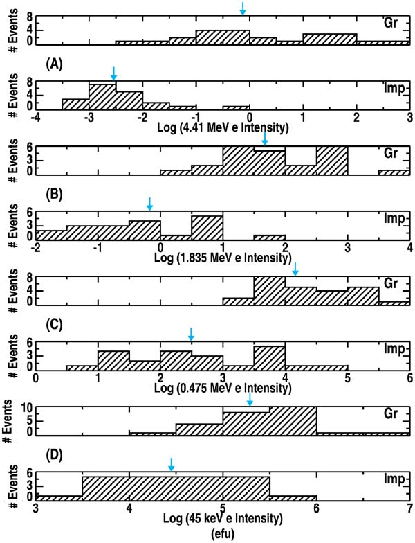
Figure 7. Histograms of electron intensity at 4.41 MeV (a), 1.835 MeV (b), 0.475 MeV (c), and 45 keV (d), for the gradual and impulsive SEP events in Tables 1 and 2. Median values of these parameters are marked by arrows.
Download figure:
Standard image High-resolution image
Figure 8. Histograms of median "electron yields" for 4.41 MeV (a), 1.835 MeV (b), 0.475 MeV (c), and 45 keV (d) electrons, for the gradual and impulsive SEP events in Tables 1 and 2. Median values are marked by arrows.
Download figure:
Standard image High-resolution image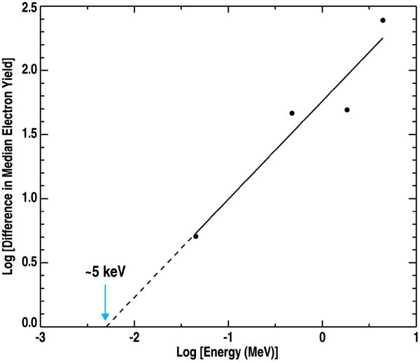
Figure 9. Difference between median "electron yields" of impulsive and gradual SEP event groups as a function of electron energy. A least-squares fit through the four data points (taken from Figure 8) extrapolated to zero difference gives an intercept energy of ∼5 keV.
Download figure:
Standard image High-resolution image2.3. Type III Burst Time Profiles
Figures 10a and 10b give superposed epoch plots of the ∼1 MHz emission for the impulsive and gradual SEP events, respectively. Here, the organizing epoch time, shown by the dashed vertical line, was taken to be the time of the maximum growth rate of the 1–8 Å time profile. The cross-hatched area in each plot indicates the times for which the ∼1 MHz emission of the flare associated with the SEP events was ≥2 × 10³ sfu. In both Figures 10(a) and 10(b), the event plots are ordered by the time difference (ΔT) between the times of maximum growth rate and peak intensity (red vertical lines in each plot) of the SXR flare, with the topmost plot having the shortest ΔT. Zhang et al. (2001) reported that the time of rapid increase in SXR intensity marks the onset of the rapid acceleration phase of coronal mass ejections. In Figures 10(a) and 10(b), we see that this time also often corresponds to the fast rise of the ∼1 MHz burst (see Reiner et al. 2001). Zhang et al. found that the peak SXR time generally signals the end of the main acceleration phase of CMEs.
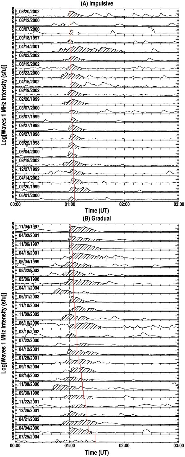
Figure 10. Superposed epoch plots of the ∼1 MHz bursts associated with the impulsive (a) and gradual (b) SEP events in Tables 1 and 2, respectively. The organizing epoch time (indicated by the dashed black vertical line) is the time of the maximum growth rate of the 1–8 Å time profile. In each event plot, the time of peak SXR emission is given by a solid red line. In both (a) and (b), the event plots are ordered by the time difference (ΔT) between the times of maximum growth rate and peak intensity of the SXR flare, with the topmost plot having the shortest ΔT.
Download figure:
Standard image High-resolution imageWe subjectively characterized the morphologies of the ∼1 MHz events in Figure 10 as simple (S), intermediate (N), or complex (C). These radio burst characterizations are listed in Tables 1 and 2. Table 3 gives a matrix of burst and SEP (impulsive and gradual) types. The most populated cells in Table 3 are impulsive/simple (11 events) and gradual/complex (17 events), supporting the idea that complexity in large type III bursts is an indicator, albeit imperfect, of which solar flares are likely to be associated with a major SEP event and those that are not (Cane et al. 2002; MacDowall et al. 2003).
Table 3. Type III Morphology Versus SEP Event Classification
| SEP Event Classification | |||
|---|---|---|---|
| Impulsive | Gradual | ||
| Simple (S) | 11 | 1 | |
| Type III Morphology | Intermediate (N) | 6 | 7 |
| Complex (C) | 5 | 17 | |
Download table as: ASCIITypeset image
Note that for three (Nos. 8, 14, and 23 in Table 2) of the 25 gradual events, the type III emission is relatively weak. This can be seen in Figures 6 and 10(b) as well as in the daily Wind/Wave plots on the Web site. Cane et al. (2006) classified Nos. 14 (2001 November 22) and 23 (2004 July 25) as shock events but, in both these cases, the >10 MeV intensity rises above 10 pfu within 12 hours.
2.4. Associations of Gradual and Impulsive Events with Strong Coronal Shocks
As has been well documented, large gradual SEP events are highly associated with the DH type II bursts that indicate the presence of strong coronal shocks (Gopalswamy et al. 2002; Cliver et al. 2004), while even the largest impulsive SEP events typically lack such association (Cliver & Ling 2007). For the gradual events in Table 2, the rate of DH association is 96% (24/25); for the large impulsive SEP events in Table 1, the association rate is 5% (1/22).8
2.5. Reverse Study Beginning with Large ∼1 MHz Bursts
As a guide in our computer search for large radio bursts from 1997 to 2004, we used the histograms of radio burst parameters in Figure 4 and compiled an initial list of events with log (940 kHz peak intensity) ≥ 5.5 and duration ≥ 15 minutes (not integrating across short data gaps in this case). We then eliminated events due to radio noise and smaller events with integrated ∼1 MHz intensities less than 2 × 10⁶ sfu minute. We made flare associations for the remaining events, using the flare listings in Solar-Geophysical Data as well as the online EIT data in the SOHO LASCO CME Catalog.9 We identified a total of 77 bursts with associated flares from W20 to W89 (after eliminating four possibly "masked", i.e., high pre-event background events without clear fresh SEP injections). The relationship of these bursts to DH type II bursts and large (≥1 pfu, in hourly averages) > 30 MeV proton events is shown in Table 4 where it can be seen that if a large favorably-located ∼1 MHz type III burst is associated with a DH type II, then it has a 10 times greater probability (57% (15/26) versus 4% (2/51)) of being followed by a significant > 30 MHz proton event than if it lacks such DH type II association. The two large > 30 MeV proton events that lacked associated DH type II bursts occurred on 2002 February 20 (see Footnote 3) and 2002 August 22 (No. 19 in Table 2). Both of these events were associated with metric type II bursts, with durations of ∼15 minutes and ∼10 minutes, respectively.
Table 4. >30 MeV Proton Event Association Versus DH Type II Association for a Sample of Large Favorably Located (W20–W89) Type III Bursts from 1997 to 2004
| >30 MeV Proton Event (≥ 1 pfu) | |||
|---|---|---|---|
| YES | NO | ||
| DH II | 15 | 11 | |
| Largea Type III Burst | |||
| No DH II | 2 | 49 | |
Note. aLog[Sp(940 kHz)] ≥ 5.5, where Sp(940 kHz) = peak radio intensity at 940 kHz; 940 kHz duration ≥ 15 minutes; integrated 940 kHz intensity ≥ 2 × 10⁶ sfu minutes.
Download table as: ASCIITypeset image
As a byproduct of this exercise, we determined that the largest solar ∼1 MHz radio burst during this period (in terms of both peak (6.3 × 10⁶ sfu) and integrated (3.17 × 10⁷ sfu minutes) intensity) occurred on 1998 September 6. This burst was associated with an impulsive C2.9 subflare (0025 UT; S20W31) with > 10 MeV proton intensity ∼0.1 pfu. The four next largest bursts in terms of integrated intensity occurred in association with gradual SEP events on 2000 July 14 (3.08 × 10⁷ sfu minutes), 1997 November 6 (2.50 × 10⁷ sfu minutes; No. 2 in Table 2), 1997 April 7 (2.49 × 10⁷ sfu minutes), and 1998 May 2 (2.39 × 10⁷ sfu minutes). Besides No. 2, four other ∼1 MHz bursts, associated with gradual events in Table 2 (Nos. 1, 3, 7, and 19), and three bursts (Nos. 2, 15, and 22), associated with the impulsive events in Table 1, had integrated ∼1 MHz intensities greater than 107 sfu minutes.
3. CONCLUSION
3.1. Summary
This study was motivated by the finding that certain large and, therefore, presumably gradual SEP events had Fe/O ratios and charge states at energies above 10 MeV amu−1 that were similar to those found in impulsive events. Two explanations were proposed to account for this behavior: (1) flare-dominated SEP acceleration at high energies (Cane et al. 2002, 2003, 2006) and (2) variation of shock geometry and seed particle population (Tylka et al. 2005, 2006; Tylka & Lee 2006). To test the first hypothesis, we considered samples of well-defined impulsive and gradual SEP events. Based on the work of Cane et al. (1981, 2002), we surmised that peak > 30 MeV proton intensity should scale with the time-integrated intensity of type III emission, the characteristic emission of flares (or of the impulsive phase of fully-developed flares). Confirmation of this expectation would support the flare-dominated acceleration of high-energy SEPs; failure to confirm would raise questions about, or cast doubt upon, the flare hypothesis. We based our study on two samples of events: a well-defined sample of classic impulsive flares, as defined by enhancements of Fe and trans-Fe elements (Reames & Ng 2004), and a sample of large gradual SEP events. If the peak > 30 MeV proton intensity scales with type III burst energy, we would expect the "proton yields" (defined as the peak proton intensity of an SEP event divided by the integrated ∼1 MHz intensity of its associated flare) of the two groups of events to be comparable. This expectation was not met.
Large impulsive and gradual SEP events exhibit dramatic differences in their ∼1 MHz radio burst proton yields. For > 30 MeV protons, the proton yield of ∼1 MHz bursts associated with a sample of large gradual events was more than 102 times that for bursts linked to a sample of large impulsive SEP events. Thus, the large > 30 MeV proton intensities observed in gradual events do not appear to result from any simple scaling up of the associated flare-resident acceleration process, as parameterized by the energy released in its characteristic type III emission. Median electron yields in the gradual events are also higher, and only approach those for impulsive events at the lowest observed energies (4.41 MeV (∼250 times higher), 1.835 MeV (∼50), 0.475 MeV (∼45), 45 keV (∼5), and ∼5 keV (1, extrapolated)), corresponding to the electrons that excite type III emission.
The radio bursts associated with the SEP events in both Tables 1 and 2 contain representatives of the largest ∼1 MHz radio events that the Sun is capable of producing (integrated intensities ∼107 sfu minutes; based on cycle 23, Section 2.5). Thus, the limit of > 10 MeV SEP production by the flare-resident acceleration process appears to be less than 10 pfu, in comparison with the observed maximum SEP intensity of ∼104 pfu in Table 2. To attribute the proton-rich (this study and Cliver & Ling 2007) large gradual SEP events to a flare process manifested by type III-l emission would require that the nature of the flare process (or processes) would change significantly as it moved from the flare impulsive phase to the delayed second stage of radio emissions (Figure 1) in order to achieve the dramatically higher proton (and high-energy electron) yields observed in these events, while retaining its capacity to produce enhanced Fe abundances. This cannot be ruled out, but it would necessitate discounting a role in acceleration of high-energy SEPs for the strong shocks observed in gradual SEP events as documented in Section 2.4 as well as by the results of our "reverse" study in Section 2.5 in which we showed that large type III bursts with an associated DH type II burst are much more likely to be followed by a significant flux of > 30 MeV protons in space than those that lack such association (57% versus 4%). Finally, we note that analysis of the 1997 November 6 event (Krucker et al., 1999), one of the four events reported by Cohen et al. (1999b) that prompted a re-examination of the standard two-class picture of SEP events, gave evidence of two acceleration processes: one process producing < 25 keV electrons that was closely tied to the intense type III burst observed in this event, and a delayed process responsible for protons and high-energy electrons.
3.2. Discussion
Given the failure to find support—via our yield analysis—for the picture that a flare-resident particle acceleration process dominates large > 25 MeV SEP events (Cane et al. 2003), the simplest explanation for our results is that proton and high-energy electron acceleration in large gradual SEP events are primarily due to shock acceleration (Gopalswamy et al. 2002; Cliver et al. 2004; also Sections 2.4 and 2.5 of this study). The theory of particle acceleration by shocks at the Sun is well developed and recent advances (Tylka et al. 2005, 2006) have indicated that the evidence for flare particles in certain large SEP events (which provoked the current debate) can be accommodated in the shock scenario when shock geometry and seed particles (also see Mewaldt et al. 2006 and Cliver 2006) are taken into account. Tylka & Lee (2006) incorporated these ideas into an analytic shock model that provided a quantitative explanation for the Breneman & Stone (1985) charge/mass fractionation effect, a fundamental but previously unexplained aspect of SEP phenomenology.
Recently, Cliver (2008) proposed a revision, based on the work of Tylka and colleagues, of the two-class SEP classification scheme. In the modified framework, a middle column is added to the impulsive-gradual dichotomy (Reames 1993, 1999) to accommodate the large ACE SEP events with impulsive characteristics. Such events are attributed to quasi-perpendicular shocks that operate on flare suprathermals (either from previous flares or possibly (see Cliver et al. 2004) from the concomitant shock-related flare) to produce large SEP events with enhanced Fe composition and high Fe charge states. In this three-column scheme, the left-hand column represents the traditional flare (impulsive) column and the right-hand column represents the classic gradual (quasi-parallel shock) column. In brief, the proposed new scheme simply splits the old gradual event column into those caused by quasi-perpendicular and quasi-parallel shocks, respectively.
In Figure 10, we affirm the tendency for different burst morphologies between type IIIs associated with impulsive SEP events and those linked to gradual events, with the latter group having longer durations and greater complexity (Cane et al. 2002; MacDowall et al. 2003). The origins of these intense complex type III emissions remain controversial. They were initially attributed to acceleration of electrons by shocks (and called SA events; Cane et al. 1981), but subsequent detailed studies have provided conflicting results, with certain groups of authors (Kundu et al. 1990; Klein & Trottet 1994; Reiner & Kaiser 1999; Reiner et al. 2000) favoring the flare hypothesis and others (MacDowall et al. 1987; Kahler et al. 1989; Bougeret et al. 1998; Dulk et al. 2000; Klassen et al. 2002) arguing for a shock origin. Considering the support for both pictures and modern CSHKP-type models of eruptive flares (Figure 11), it seems likely that both mechanisms may play a role depending on the event. In the model in Figure 11, the CME can serve as a driver for a shock wave (Cliver et al. 1999; Gopalswamy et al. 2003; Lara et al. 2003)10 while reconnection in the wake of the CME (e.g., Cliver et al. 1986) following the flare impulsive phase could provide additional electron acceleration. This latter scenario was preferred by Cane et al. (2002) as the source for type III-l emission. While type III emission in the second (or extended) stage is missing from the classic view of a fully-developed radio burst as shown in Figure 1, Figure 10(b) shows this to be an oversimplification. Both the flare-resident process and shocks are available to accelerate electrons during this phase.
Figure 11. Standard CSHKP-type model (see Hudson & Cliver 2001) of eruptive solar flares, illustrating the two late-phase acceleration processes—reconnection leading to flare loops in the wake of the CME and CME-driven shock acceleration (taken from Cliver et al. 2004).
Download figure:
Standard image High-resolution image
In the eruptive flare model in Figure 11, a fast CME creates the second phase radio emission (via shocks and extended reconnection) of fully-developed bursts shown in Figure 1. In most events, all we see is the first phase and the type III burst has a simple profile as observed for many of the large impulsive events in Figure 10(a). This implies either no-CME or a CME in which the escaping material goes out on open field lines (Shimojo & Shibata 2000; Kahler et al. 2001) and thus neither drives a shock (Vršnak & Cliver 2008) nor is followed by reconnection.
The hypothesis that flares dominate proton acceleration above 25 MeV is practically indistinguishable from the shock hypothesis in terms of the relevant solar observables since long-duration type IIIs can be seen to be a consequence of a fast CME. As Cane et al. (2002) suggested, "... type III-l bursts result from the departure of large, fast CMEs," precisely the condition required for shock formation (Gopalswamy 2006). Thus, the presence of DH type IIs in large SEP events could be taken to be indirect support for the flare hypothesis. In this study, we moved beyond this ambiguity by attempting, and failing, to confirm what seems to be a logical consequence of the flare hypothesis advanced by Cane and colleagues—that large type III bursts should signal commensurate production of high-energy protons. It turns out that they do so only when a strong shock is present.
We thank D. Reames and A. Tylka for comments on a draft of this paper and the referee for helpful comments. A.G.L. was supported by AFRL contract FA8718-05-C-0036.
Footnotes
- 3
We excluded three SEP events from the Cane et al. (2006) list for which the hourly-averaged J (>10 MeV) peak values were less than 10 pfu. These SEP events occurred on 2001 September 15, 2001 October 19, and 2002 February 20.
- 4
Available at http://lep694.gsfc.nasa.gov/waves/waves.html
- 5
Data available at http://spidr.ngdc.noaa.gov/spidr/index.jsp
- 6
The galactic background is subtracted from the GOES data but not from the SIS data. The SIS proton data are available on the ACE Web site at http://www.srl.caltech.edu/ACE/ASC/browse/view_browse_data.html
- 7
Both the COSTEP and EPAM electron data are available on the Coordinated Data Analysis (CDA) Web site at http://cdaweb.gsfc.nasa.gov/cdaweb/istp_public/. COSTEP data for dates after 2002 January can be found at http://sohodata.nascom.nasa.gov/cgi-bin/gui
- 8
- 9
These data are available at http://cdaw.gsfc.nasa.gov/CME_list/
- 10
A quasi-parallel shock is depicted. Note that lateral expansion of the CME could drive a quasi-perpendicular shock.